CHT Analysis on Exhaust Port

Aim : CHT analysis on exhaust port

Objectives :

• Give a brief description of why and where a CHT analysis is used.
• Maintain the y+ value according to the turbulence model and justify the results.
• Calculate the wall/surface heat transfer coefficient on the internal solid surface & show the velocity & temperature contours in appropriate areas.
• How would you verify if the HTC predictions from the simulations are right? On what factors does the accuracy of the prediction depend on?

Theory :

1. Introduction:

• The main difference between thermodynamic analysis and heat transfer analysis is that in thermodynamic , we deal with system in equilibrium i.e. to bring a system from one eqb. State to another equilibrium state how much heat required is the main criteria. While in heat transfer analysis, we evaluate at what rate this change of system occurs by calculating rate of heat transfer in (J/s or Watt).
• Heat transfer is known as the flow of thermal energy from one region to another region occupied by any matter (solids and fluids) where the rate of heat transfer is proportional to the temperature difference between the regions/matters.
• Conjugate heat transfer (CHT) is used to describe the variation of temperature between the solids and fluids due to the exchange of thermal energy between them.

2. Modes of heat transfer :

• There are 3 ways of modes of heat transfer

1. Conduction
2. Convection
3. Radiation

2.1. Conduction :

• Conduction is the mode of heat transfer which generally occurs in solids due to temp difference associated with molecular lattice vibration energy transfer and also by free electron transfer.
• The reason behind all electrically good conductors are also in general good conductors of heat is that the presence of abundant (i.e. plenty) number of electrons available in the outermost orbit of atoms.

Ex : All metals.

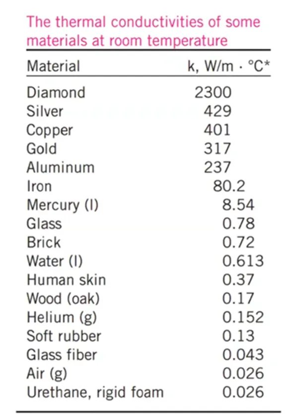
• Notable exception to the above statement is Diamond (K=2300 W/m-K). The highest conductivity of diamond is due to perfect crystalline molecular lattice structure.

2.1.1. Fourier’s law of conduction :

• It states that,” the rate of heat transfer by conduction along a given direction is directly proportional to the temp gradient along that direction and is also directly proportional to the area of heat transfer lying perpendicular to the direction of heat transfer.”

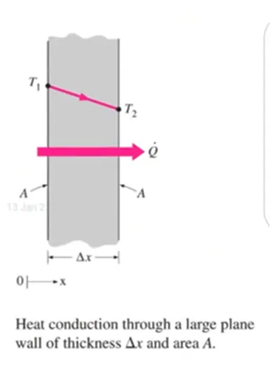
i.e. `underset(x)q prop(dT)/(dx)`

And `underset(x)q prop A`

Now by combining these equations we can write as

`underset(x)q= -KA(dT)/(dx)`

Where,

K= Thermal conductivity (W/m-K)

A = Normal surface area (m²)

`(dT)/(dx)` = Temp gradient

q_x = Conductive heat transfer (Watt)

• Here the negative sign denotes heat transfer in the direction of decreasing temperature.
• Thermal conductivity is the measurement of materials ability to conduct heat.

2.1.2. Thermal conductivity (K (W/m-K)) :

• The thermal conductivity of a material is defined as,’It is a thermophysical property of a material which tells about the ability of the material to allow the heat energy to get conducted through the material more rapidly.’
• Insulators have very low value of ‘K’ .so there can prevent heat transfer rate.

Ex: asbestos, refractory bricks, glass wool, polyurethane foam etc.

• It can also be defined as, “the rate of heat transfer through a unit thickness of the material per unit area per unit temperature difference.”
• The unit for K= W/m-K or W/m-`overset(o)`C
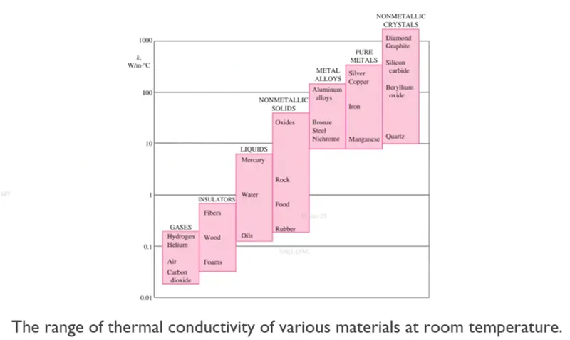
• The thermal conductivity of a some materials at a room temp is given as follows

2.1.3. Thermal diffusivity(`alpha`) :

• It is defining as, “ It is a thermophysical property of a material, as the ratio between thermal conductivity of a material and its thermal capacity.”

`alpha=(K)/(rhounderset(p)C)` ,(m²/s)

Where,

ρ = Density of material (kg/m³)

C_p = Sp. Heat capacity of that (J/kg-K)

K = thermal conductivity of material (W/m-K)

ρC_p = thermal storage capacity of material

• Thermal diffusivity of a material tells about the ability of a material to allow the heat energy to get diffused or passed through the material more rapidly.
• Higher the conductivity of the material and lesser its heat capacity , more the value of thermal diffusivity.
• Thermal diffusivity of gases is more compared to thermal diffusivity of liquids.

Ex : α_air > α_water (as K_air < K_water and ρCp_air << ρCp_water )

• High value of K will result a faster energy transfer through a material.
• Low value of Cp represents lesser amount of heat moving through the material will be used for raising the temperature and more of it will be available for transferring.

2.2. Convection :

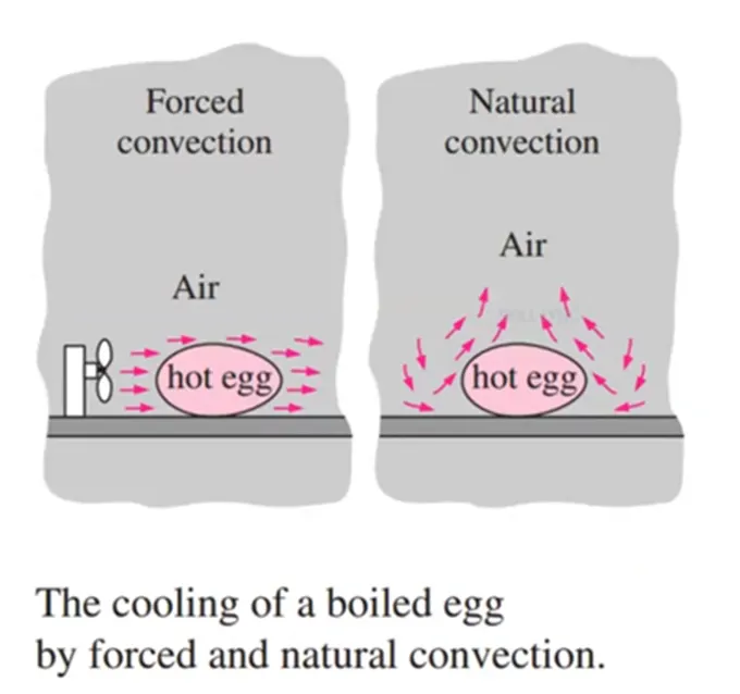
• Convection is the mode of heat transfer which generally occurs between a solid surface and the surrounding fluid due to temp difference associated with macroscopic bulk motion of the fluid transporting thermal energy in the form of enthalpy.
• In case of forced convection heat transfer this motion of fluid is provided by an external agency like a fan or blower or a pump where as in free convection heat transfer the motion of the fluid occurs naturally due to buoyancy forces arising out of density changes of fluid because of its temperature.

2.2.1. Newton’s law of cooling :

• The law states that, “the rate of heat transfer by convection between solid body and surrounding fluid is directly proportional the temp difference between them and also directly proportional to the area of contact or area of exposure between them.”

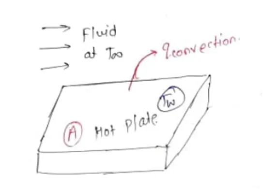
i.e. `underset(conv)q prop (underset(w)T-underset(oo)T)`

And `underset(conv)qprop A`

Therefore, `underset(conv)q= hA(underset(w)T- underset(oo)T)`

Where,

h= convective heat transfer coe. (W/m²-K)

A= surface area of a solid body where fluid comes in contact (m²)

T_w = plate temp (K)

`underset(oo)T` = fluid or ambient temp (K)

• The convective heat transfer coe.(h) is not a property of the fluid. It is experimentally determined parameter whose value depends on all the variables influencing convection such as the surface geometry, the nature of the fluid motion, the properties of the fluid and the bulk fluid velocity.
• Typical values of h are given in table

Sr. no	Type of convection	h(W/m2-K)
1	Free convection in gases and vapours	3-25
2	Forced convection in gases	25-400
3	Free convection in liquids	250-600
4	Forced convection in liquids	600-4000
5	Condensation in heat transfer	3000-25000
6	Boiling heat transfer	5000-50000

2.2.2. Nusselt number:

• It is the ratio of convective heat transfer to conductive heat transfer within a fluid region.

`Nu="Convective heat transfer"/"Conductive heat transfer"`

`Nu=h/(K/L)=(hL)/K`

Where,

h = convective heat transfer coe. (W/m²-k)

K = thermal conductivity of a fluid (W/m-k)

L= thickness of a plate (m)

• Nusselt number denotes the increase in heat transfer through a fluid layer caused by convection, relative to conduction.
• When a fluid is motionless (i.e. no bulk motion), conduction will be the dominating mode of heat transfer (Nu=1).
• When a fluid is in bulk motion, the convection will be higher.

2.2.3. Prandtl’s number:

• It is the ratio of momentum diffusivity to thermal diffusivity.
• It compares the velocity boundary layer thickness to the thermal boundary layer thickness (which boundary layer is thicker).

`Pr="Momentum Diffusivity"/"Thermal Diffusivity"`

i.e. `Pr="Velocity boundary layer thickness"/"Thermal boundary layer thickness"`

i.e. `Pr= nu/α= (μ/ρ)/(K/(ρC_p ))=(μC_p)/K`

Where

`nu` = Kinematic/momentum diffusivity (m²/s)

α = Thermal diffusivity (m²/s)

µ = dynamic viscosity (Pa-s)

C_p = sp. Heat (J/kg-K)

• Prandtl number is a dimensionless number.
• Prandtl number for gases is about 1, for water it is in the order of 10.
• It is 0.01 for liquid metals and 10⁵ for heavy oils.
• For air, Pr=0.65 - 0.71
• Local conv. Heat transfer coe. For laminar boundary layer over a flat plate can be determined from following empirical equation as,

`Nu= (hL)/K=0.664 Re^0.5 Pr^0.33`

• For fully developed turbulent flow through pipes or ducts , the heat transfer coe. Can be calculated as,

`Nu= (hD)/k=0.023 Re^0.8 Pr^n`

Where,

n= 0.4, for heating of the fluid

n= 0.3, for cooling of fluid.

2.2.4. Reynolds number :

• The Reynolds number is a dimensionless number, named after the Osborne Reynolds , defined as the ratio of inertia forces to the viscous forces. Mathematically it is given as,

Re=`"Inertia force(Fi)"/"viscous force (Fv)"`

i.e. Re=`= (ρVD )/μ = (VD)/ν`

where ,

ρ = density of fluid (kg/m³)

V = velocity of fluid (m/s)

D or L = diameter of pipe or characteristics length of pipe (m)

μ = dynamic viscosity of fluid (N-s/m²)

`nu` = kinematic viscosity of fluid (m²/s)

• Significance :
  • Reynolds number is used in the forced convection. Forced convection is a type of heat transfer in which fluids are forced to move in order to increase the heat transfer.
  • Reynolds number is used to predict the flow patterns in the different fluid flow situation. At a low Reynolds number, the flow tends to be laminar flow, while at a high Reynolds number flow tends to be turbulent flow.
• Laminar flow :
  • If a fluid travels smoothly in a regular path then flow is called as laminar flow. If flow is to be called laminar flow when the following conditions satisfy.
    • For internal flow, Re < 2000.
    • For external flow, Re < 10⁵.
• Turbulent flow :
  • If a fluid flows in an irregular path instead of regular path, then it is called as turbulent flow. The flow to be called as turbulent flow when following conditions occurred.
    • For internal flow, Re > 4000
    • For external flow, Re > 5 x 10⁵.

2.3. Radiation :

• Radiation is the mode of heat transfer which does not required any material medium for the propagation and hence occurs by electromagnetic wave propagation travelling with the speed of light.
• This radiation mode of heat transfer completely predominant over conduction and convection particularly when the temp difference is sufficiently large.

2.3.1. Stefan-Boltzmann’s law of radiation :

• The law states that, “ The radiation energy emitted from the surface of the black body per unit time per unit area is directly proportional to the fourth power of the absolute temp of the body.”

`underset(b)E prop T^4`, (where T in K)

`underset(b)E=sigmaT^4`, (J/m²-s)

Where,

σ= Stefan-Boltzmann’s constant = 5.67 * 10^-8 W/m²-K⁴.

3. Introduction to CHT analysis :

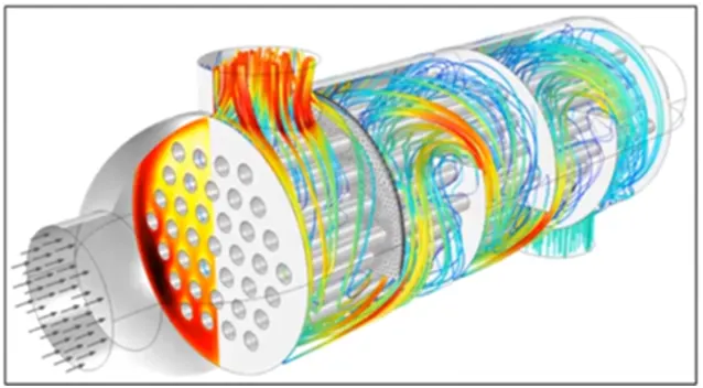
• The word CHT stands for ‘Conjugate heat transfer’.
• CHT analysis is the analysis of heat transfer between a solid and fluid domain by exchanging the thermal energy at interface between them.
• Here the conjugate means there is heat transfer takes place through two modes as conduction and convection simultaneously.
• This analysis is used because whenever thermal energy transfer takes place through 2 modes of heat transfer so we have to simulate and find out the heat transfer coe., maximum temp, avg surface temperature, convective heat transfer coe., conductive heat transfer etc.
• This analysis is generally used in the analysis of heat transfer in exhaust ports, boilers, engines, heat exchangers, regenerators, furnace walls etc.

4. Maintaining Y-plus :

• Y-plus is a non-dimensional number.
• Y is a distance from wall which is measured in terms of boundary layer thickness.
• Here, we have to maintain Y-plus w.r.t. turbulence model.

Ex: For K-omega-SST model, the range of Y-plus is 0-5 and for K-epsilon model it ranges as 30-300.

• In this case, we have to maintain the Y-plus in the range of 0-5 to capture the near wall viscous effects will gives accurate results at near the wall.

5. Boundary layer concept :

• When any viscous flow flows over a surface, a region of slow-moving flow called boundary layer develops.
• Inside the boundary layer, there is a strong velocity gradient and U varies non-linearly.

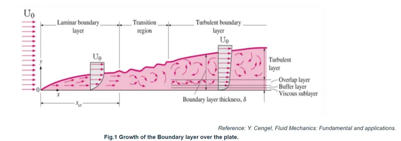
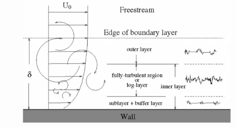
• The boundary layer comprises of –
  • Inner layer i.e. 10-20% of total boundary layer thickness
  • Laminar sub-layer closest to the wall where viscous force dominates
  • Buffer layer where viscous and turbulent forces are of similar magnitude.
  • Log-law layer where turbulent forces dominates and velocity exhibits logarithmic variation.
  • Outer layer (law of the wake) where inertia forces dominate and flow is free from viscous effects.

Modelling approach :

1. Pre-processing methods :

1.1. Geometry :

• Open the ansys workbench application.
• Drag the fluid flow (fluent) to the project schematic.
• Now right click on geometry -> import model -> browse model -> select the required cad file and importing of cad model is done.
• Again right click on geometry and select edit geometry by using spaceclaim.
• The models looks as

• Now extract the volume. For that goto prepare -> extract the volume-> select edges to extract the fluid volume

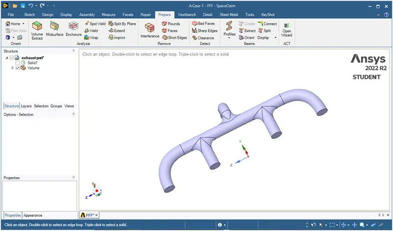
• After that enabled share topology. For that goto workbench -> share -> click on green tick symbol.

• Now we are done with geometry cleanup. So we are going for meshing.

1.2. Meshing :

• Open mesh application.
• Lets gives names to the selected faces as shown below

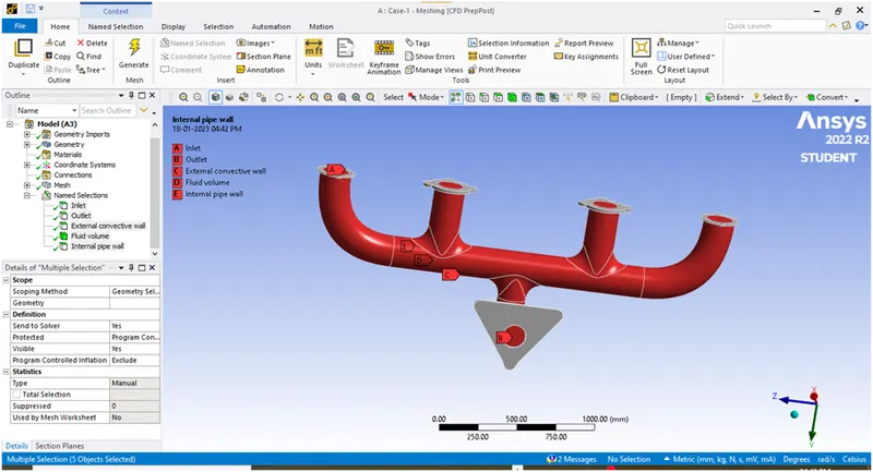
• Lets create a mesh with 150mm size i.e. base line mesh

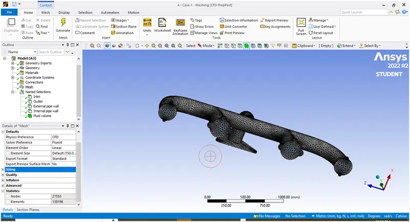
• Let add inflation layer to capture the near wall viscous effects. For that first of all calculate first layer thickness using online y-plus calculator.

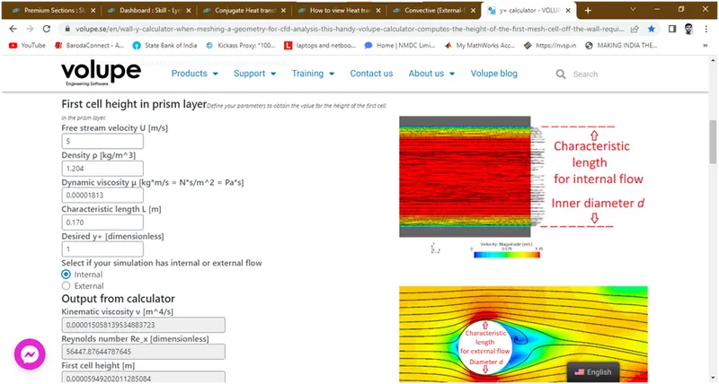
By giving inputs as v=5m/s, characteristics length=0.170mm, y-plus=1, we are getting first cell height=0.06mm.now create an inflation layer. For that right click on mesh -> insert -> inflation -> select body where to develop inflation layer -> select boundary as internal pipe wall -> select first layer thickness -> and gives value=0.06mm -> no. of layers =19 -> growth rate=1.3 for smooth volume transation -> right click on mesh -> click on update.

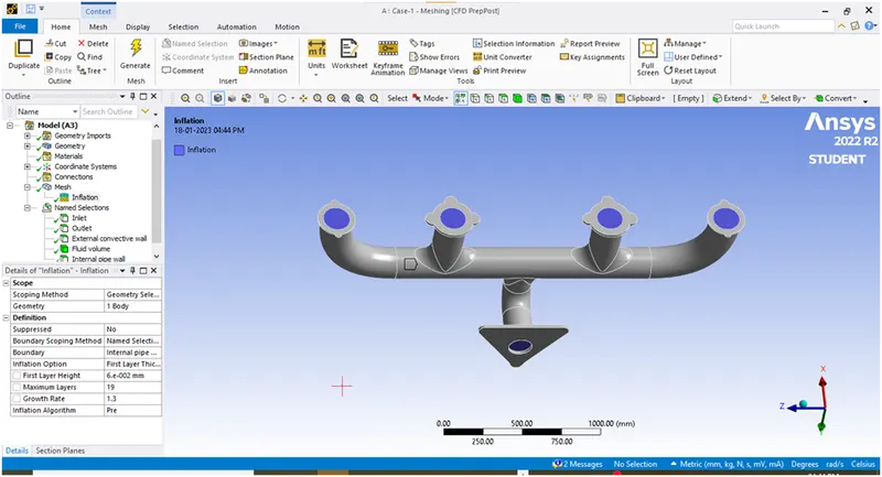
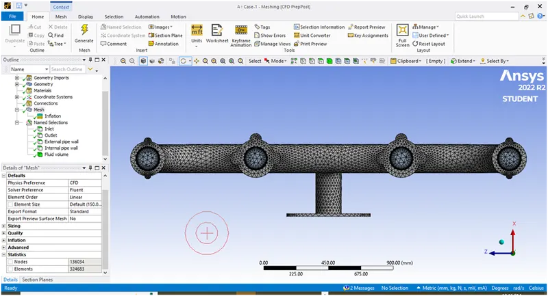
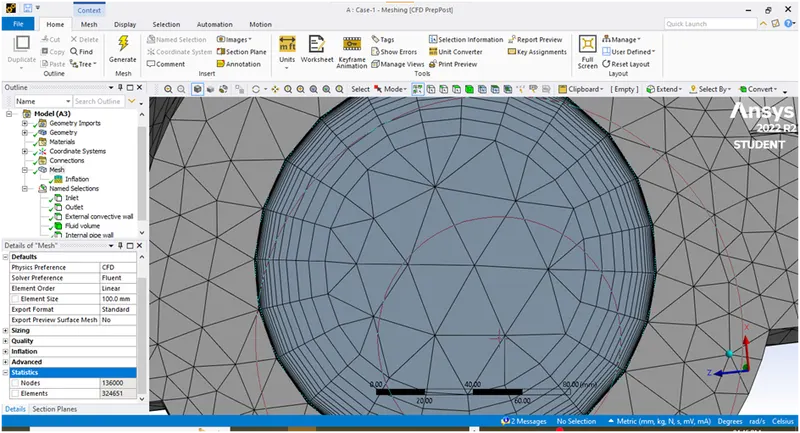
• Lets right click on mesh -> click on update to translate the data to fluent.
• Then close the meshing.
• Now pre-processing has been done. So lets we are going for post-processing methods.

2. Post-processing methods :

2.1. Setup :

• Open ansys fluent
• Click on double precision and no. of processors=4 and then click on start. The fluent application will open and the GUI looks as follows

• Now setup the fluent as shows below in table

Sr. no.	Parameters	Setup conditions
1	Solver	Pressure based
2	Solver time state	Steady state
3	Energy model	ON
4	Turbulence model	K-omega-SST model
5	Material	Fluid-Air(default) Solid- aluminium(default)
6	Boundary conditions	Inlet : velocity inlet(V=5m/s & T=700K) Outlet : pressure outlet(T=300k) External wall convection : convection(h=20W/m2-K) Internal solid surface : wall BC
7	Solving method	coupled

• Now create new report as surface-htc.
• Initialize the solution-> select hybrid initialization method
• Now run the calculation for convenient iterations.
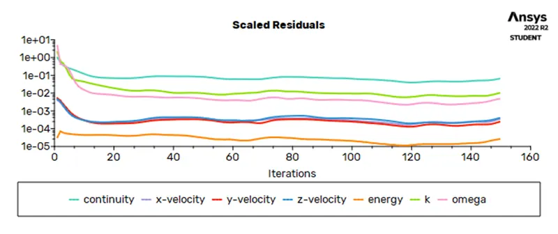
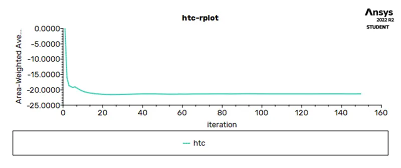
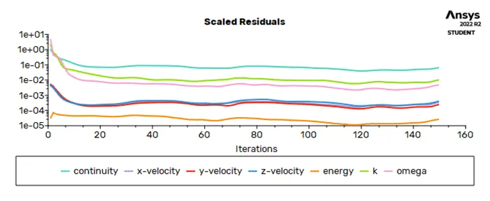
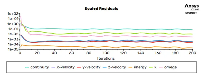
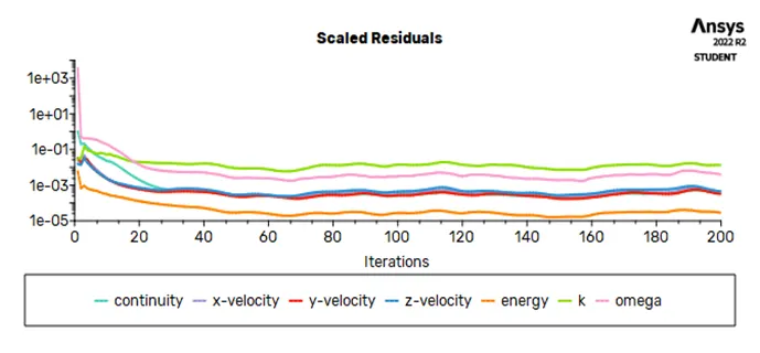
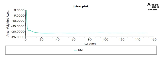
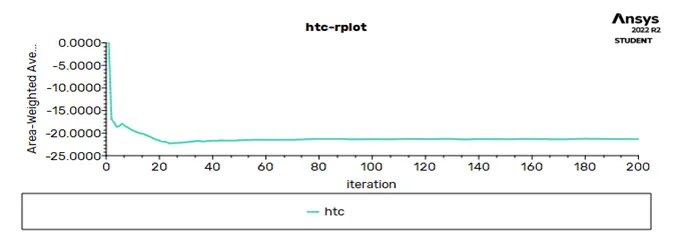
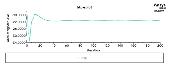
• Now plots the residual plot and htc plot as shown below

• Now export the solution data to cfd post taking into account variable as surface heat transfer.
• Close the fluent

1.2. Results :

• Open cfd-post
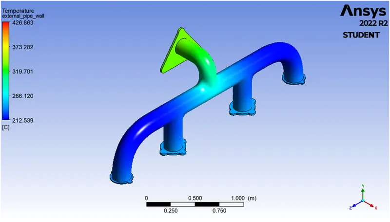
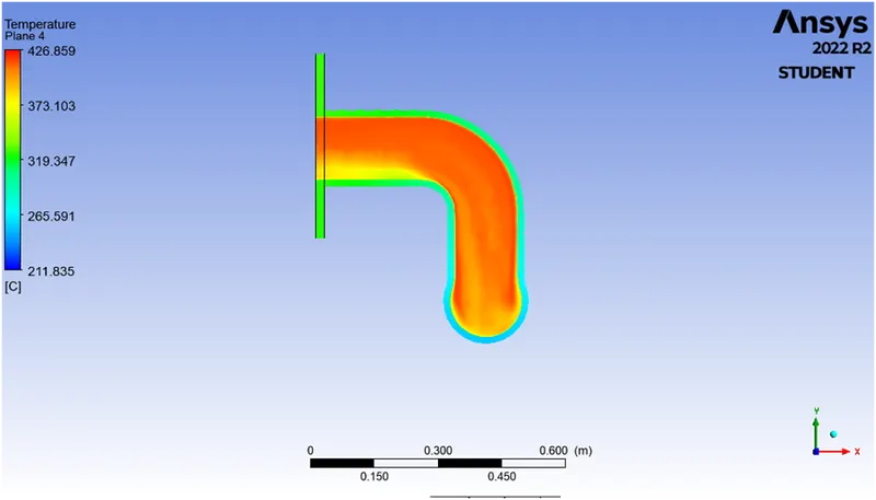
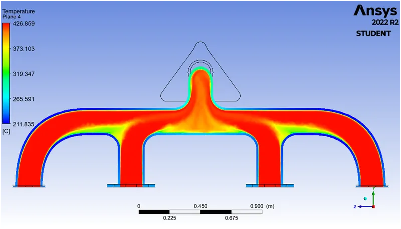
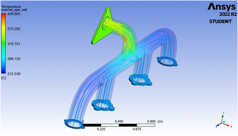
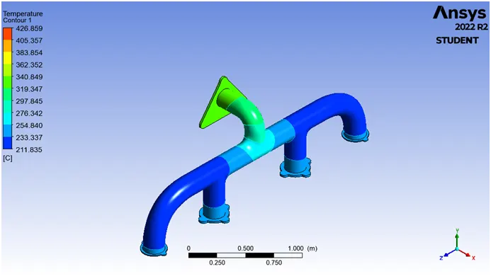
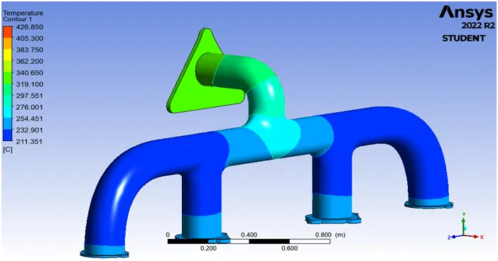
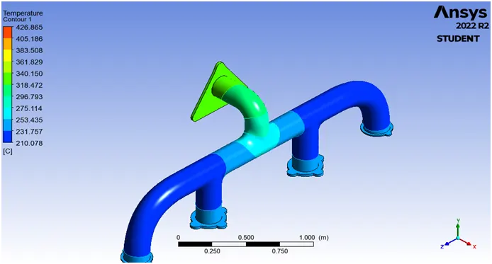
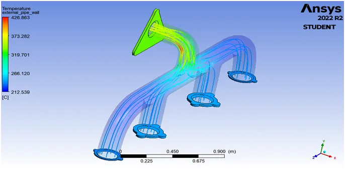
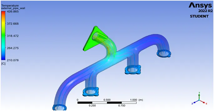
• Plot a temperature contour plot at external pipe wall as shown below

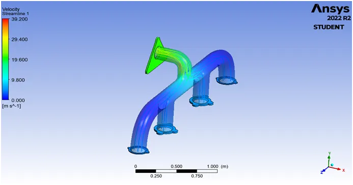
• Plot velocity streamlines at external pipe wall as shown below

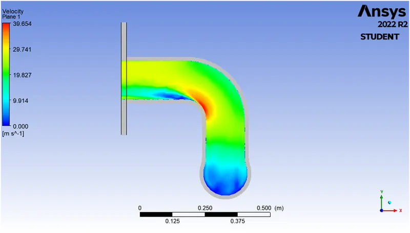
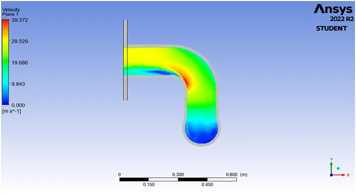
• Plot velocity contour plot at x-section xy-plane as shown below

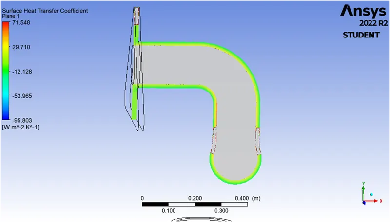
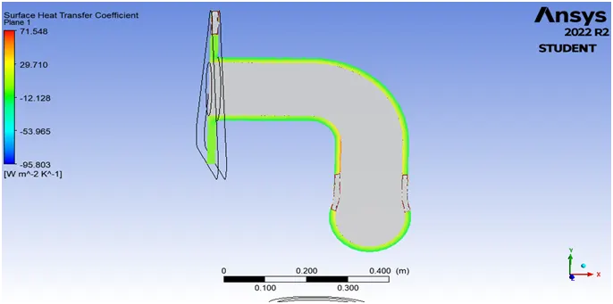
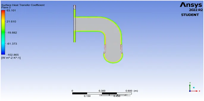
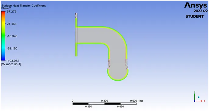
• Firstly load the results which was export from fluent and then plot surface htc contour plot at x-s/c plane i.e. xy-plane as shown below.

• Then just by changing the mesh size repeat all the procedure to get study the grid independent study and observe is mesh size affects the results or not.

3. Analytical validation :

• The properties of air is given as

V= 5 m/s

D = 0.170m

ρ= 1.225 kg/m³

µ= 1.8 * 10^-5 Pa-s

K= 0.0242 W/m-K

C_p= 1006.43 J/kg-K

• Lets calculate Reynolds number

`Re=(rhoVD)/mu`= 57,847

• Lets calculate Prandlt number

`Pr=(muunderset(p)C)/K`= 0.748

• Lets calculate Nusselt number for internal pipe flow

According to Diltus-Boelter equation

`Nu=0.023Re^0.8Pr^0.3`= 136.089

• Lets calculate heat transfer coe.

`Nu=(hD)/K`

`therefore h=(NuK)/D`

Since, = 19.372 W/m²-K

Results :

• Htc for different cases i.e. mesh independent study

SR.no	Mesh type	Mesh size	Cell counts	Heat transfer coe.(W/m2-K)
1	Base line mesh	150mm	325089	-21.316
2	Fine mesh	100mm	324903	-21.326
3	Finer mesh	50mm	325225	-21.329

• Residual plots

Sr.no	Mesh type	plots
1	Base line mesh
2	Fine mesh
3	Fine mesh

• Surface htc plot

Sr.no	Mesh type	plots
1	Base line mesh
2	Fine mesh
3	Fine mesh

• Temperature contour plots for external pipe

Sr.no	Mesh type	plots
1	Base line mesh
2	Fine mesh
3	Fine mesh

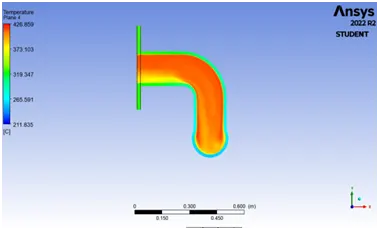
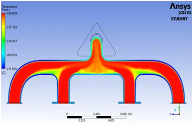
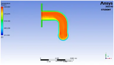
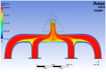
• Temp contour at planes

Sr.no	Mesh type	plots
		XY-plane	YZ-plane
1	Base line mesh
2	Fine mesh
3	Fine mesh

• Velocity contour plots

Sr.no	Mesh type	plots
1	Base line mesh
2	Fine mesh
3	Fine mesh

• Velocity streamlines

Sr.no	Mesh type	plots
1	Base line mesh
2	Fine mesh
3	Fine mesh

• Surface htc contour plots

Sr.no	Mesh type	plots
1	Base line mesh
2	Fine mesh
3	Fine mesh

Conclusion :

• Comparision and validation of htc

	Numerically	Analytically
Heat transfer coe.(h (W/m2-K))	-21.33	19.372

From above comparison we can said that with approx 6% error our htc calculated numerically is validates. Here negative sign represents there is a heat rejected by fluid.

• From result-1 i.e. mesh independent study, we can say that, the solution is independent on the mesh size and the base line mesh gives correct results.
• From residual plots and surface htc plot, we can say that, the solution gets almost converged i.e. the values reached steady state around 80 iterations.
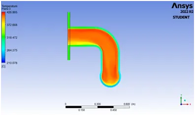
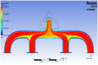
• From temp contours we can say that, at inlet the temp is more but as fluid/air moves towards outlet there is a convective heat transfer happens. Due to this the temp of air at external pipe wall decreased but near to the outlet we can see that the temp is increased slightly. This is because of the there is mixing of fluid takes place which are come from 4-inlets. Now to balance the energy equation the temp is increased slightly at outlet.
• From temp contours at planes we can see that, how the temp distribution of hot fluid which flows inside the pipe takes place. By changing mesh size there is no change in the results and plots.
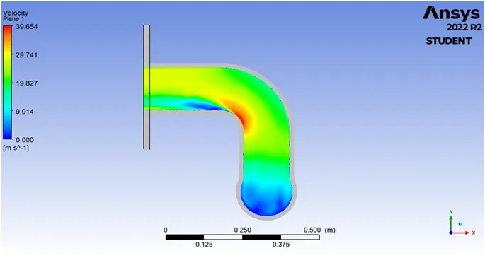
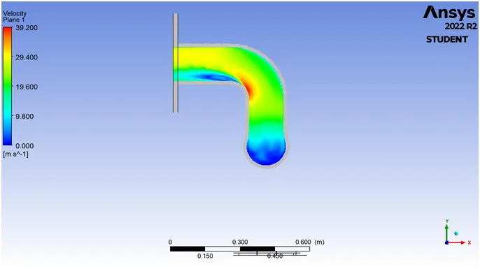
• From velocity contours and streamlines, we can see that at L-section/ joint at outlet the velocity is increased compared to inlets. Now this is due to mixing of fluids takes place which are come from multiple inlets and flows out through a single outlet. Now to fulfil the continuity equation and catch a constant speed and gets mixed properly the speed was increased. Also at bend we can see slight increase in velocity due to pipe bend effect.
• From surface htc contour plots, we can see that the surface heat transfer occurs only at boundary due to boundary layer phenomenon. There is a thermal boundary layer thickness present which causes restrictions to the fluid flow and according to Maxwell conditions/no slip condition there is frictional force acting due to shear force and in the pipe wall the boundary layer phenomenon occurs around 2-3% thickness of diameter from boundary. And in this case the boundary layer thickness is around 7mm. now at corner we can see that there is a slightly increased in surface htc is due to bend phenomenon in the pipe.