Week 4 - CHT Analysis on Exhaust port
What is CHT analysis-
Conjugate heat transfer (CHT) is a method of analysis which is used to measure the heat transfer between the body and the fluid flowing over or inside it as a result of interaction between two objects. The Conjugate Heat Transfer analysis type allows for the simulation of heat transfer between solid and fluid domains by exchanging thermal energy at the interfaces between them.
Understanding the intricate heat transfer mechanisms and the relationships between those mechanisms can help the components working in these conditions operate better and last longer.
Conjugate heat transfer analysis gives a thorough understanding of the velocity distribution and fluid heat transfer mechanism, such as in engines, as well as the temperature distribution in solids and fluids.
Why CHT analysis?
Simulating the conditions is faster and more economical than building and testing actual prototypes.
It is used to test out complex geometries and scenarios, such as in automobile or power plant components.
Iterating for different conditionss is quick and easy with immediate results.
Any form of region combination, including solid-fluid and fluid-fluid, can be simulated.
Where CHT analysis is used-
Automobile sector for componenets such as turbo charger, intercoolers and exhaust systems.
HVAC systems
Power plant systems.
Electronics sector
Modeling and simulation setup: (Case-1)
I extracted the inner volume from the model using the volume extract command. Now the inner volume has been extracted. 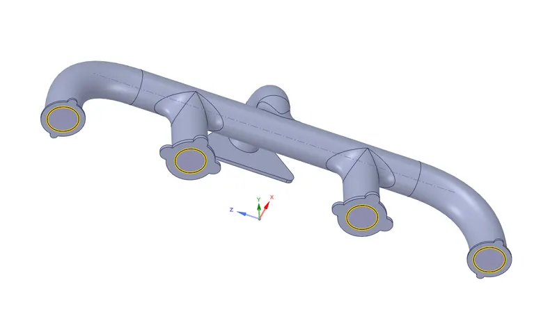
This new volume is then moved to a new component and grouped with the pipe model.
To create a conformal mesh, I enabled shared topology in the properties tab, and in workbench tab, I selected the Share Prep option. This will allow me to create a common interface with the pipe and inner volume.
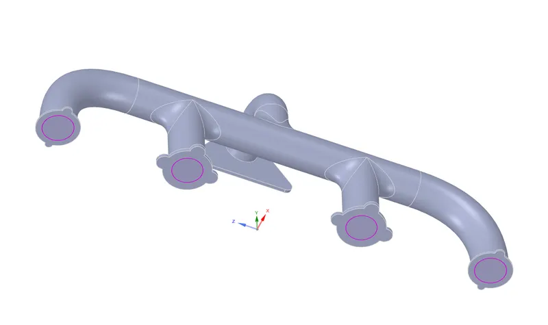
Before meshing the model, I created named selections for inlet, outlet and walls. Then for meshing I first created mesh with defualt size.
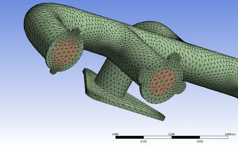
Next In Fluent, I first performed the mesh check. The I setup the simulation conditions.
The solver type is pressure based and time is steady state. The viscous model I selected as k-Epsilon model. For the material, the fluid was selected as air and the pipe material was selected as Aluminium.
Boundary conditions-
Inlet velocity-5 m/s
Tempereture- 700°C
Outlet Gauge presure- 0 pa
Then I intialized the setup and created a temperature contour plot at inlet and outer walls.Then I ran the simulation for 550 iterations.
Results:
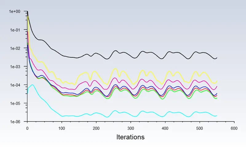
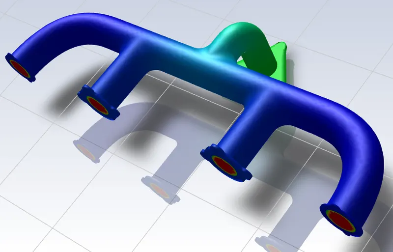
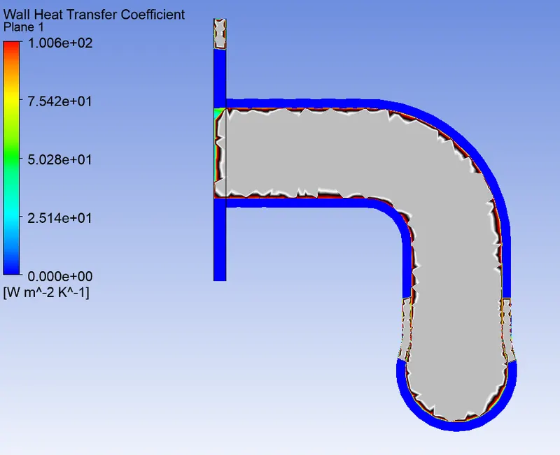
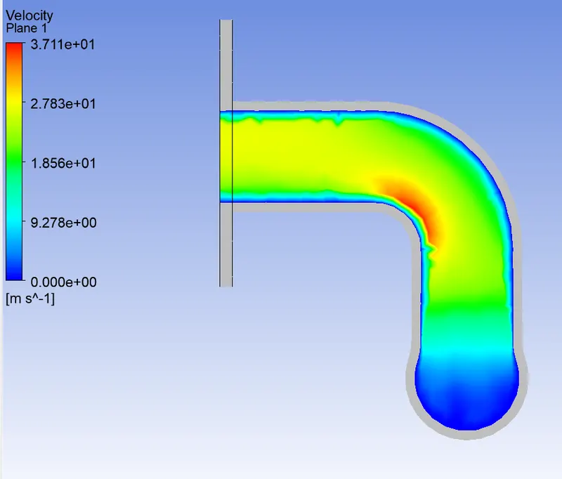
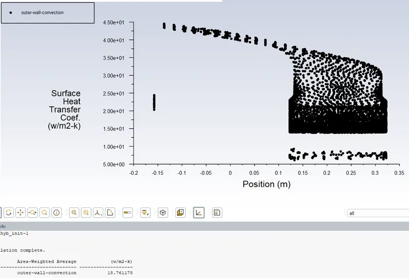
The outer wall convection value is 18.7611
Modeling and simulation setup: (Case-2)
For the second case I refined the mesh by adding inflation layers and reducing the mesh size to 5mm.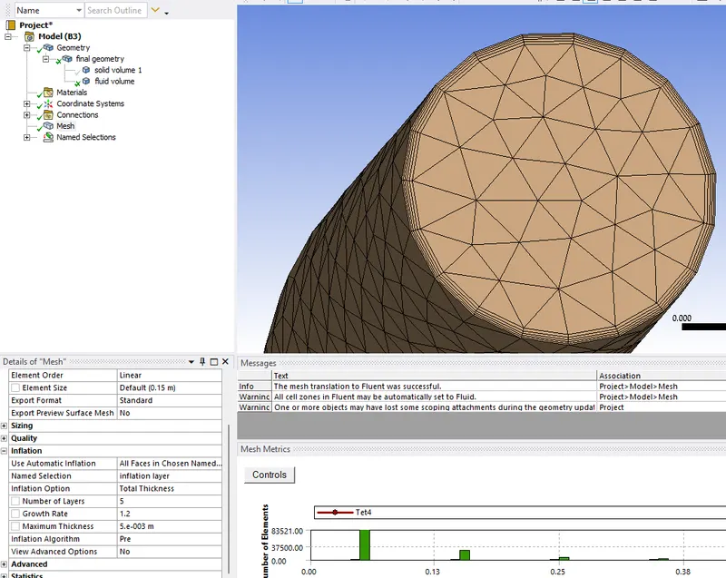
The simulation conditions were same as for case 1. I solved for 500 iterations.
Results: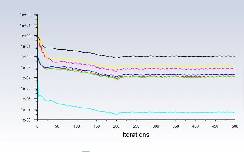
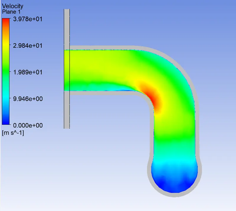
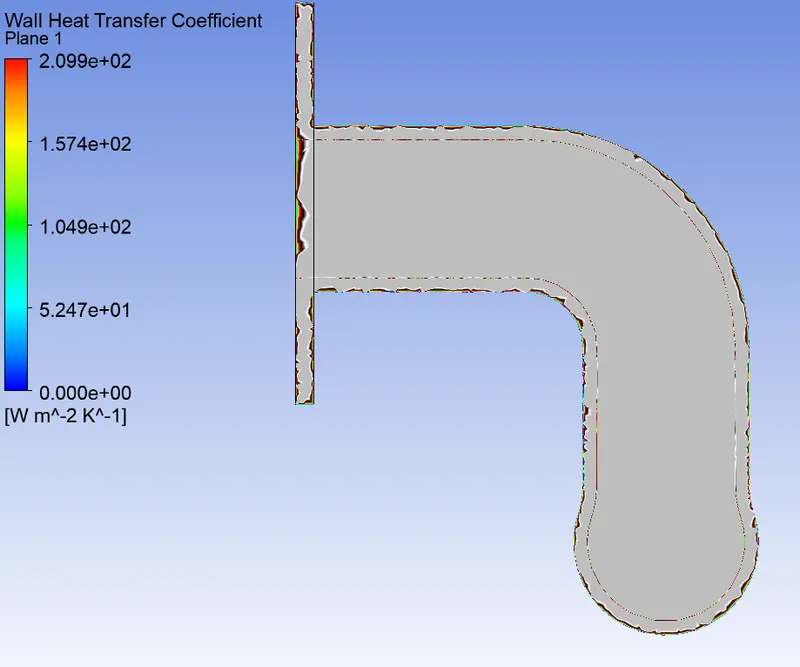
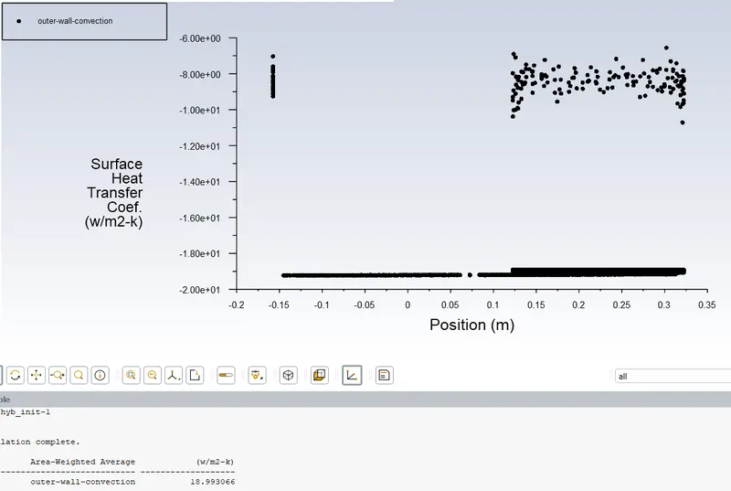
The outer wall convection value is 18.9930
Verificaton of HTC predictions:
Accuracy of the predictions depends on several things like geometry of model, mesh size and quality, Inflation layers, material type and properties, Inlet temperature and velocities and Type of solver used.
According to the Sieder Tate relation which correlates the Nu number with Re and Pr.
Nusselt no. is the function of Reynolds no. and Prandtl no.
Nu = h * k / L
Therefore h = Nu-k/L
where h = heat transfer coefficent
Nu = Nusselt number
k = Thermal conductivity coefficent
L = length
From the above equation, as the length of pipe and thermal conductivity are constant, value of h will increase as Nu increases. Therefore Nu increases as Re increases.
Most accurate way to verify our results is to validate our simulation data with published experimental data.