Week 4 - CHT Analysis on Exhaust port
Aim and its objective:
- A brief explanation of when and why a CHT analysis is employed in this challenge.
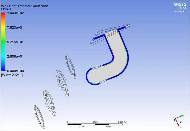
CHT Analysis on an Exhaust port is used to mimic the both fluid flow and heat transfer to a solid. - Then, on the internal solid surface, determine the wall heat transfer coefficient and display the velocity & temperature contours where necessary.
- And confirm that the HTC predictions based on the simulations are accurate as well as the variables on which the prediction's correctness depends.
Definition:
Conjugate Heat Transfer (CHT) analysis
Conjugate Heat Transfer analysis allows for the simulation of heat transfer between solid and fluid domains by exchanging thermal energy at the interfaces between them and transporting via conduction within solids and additionally via convection within fluid domains. Conjugate heat transfer analysis can accurately predict heat transfer by simultaneously solving all the relevant solid and flow field heat transfer processes. Conjugate heat transfer corresponds with the combination of heat transfer in solids and heat transfer in fluids. In solids, conduction often dominates whereas in fluids, convection usually dominates. Conjugate heat transfer is observed in many situations for example conduction through solids, free and forced convection in the gases/fluids, and thermal radiation.
- The three main modes of heat transfer:
‐ Conduction is heat transfer that occurs when a temperature difference exists across a stationary medium.
‐ Convection is the heat transfer between a surface and a moving fluid when there is a temperature difference between the two.
‐ Radiation(thermal radiation) is the emission of energy in the form of electromagnetic waves. In the absence of an intervening medium, there is net heat transfer by radiation between two surfaces at different temperatures.
Procedure:
Case 1- Baseline setup:
Simulating the flow with the Steady case 1:
Pre-processor
Geometry in space claim:
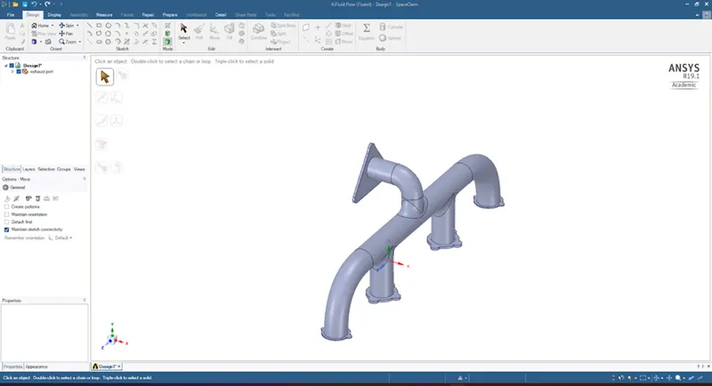
- In geometry, it has a solid part. So firstly, extract the fluid volume. To do this, the process follows
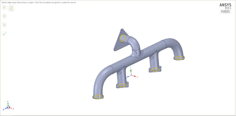
prepare -> volume to extract -> select edge selection -> then select all the edges of inlet and outlet -> to click ok. The fluid volume will be created.
- Then, after the volume has been created, change the name of the components, i.e., fluid volume to fluid and solid volume to solid.
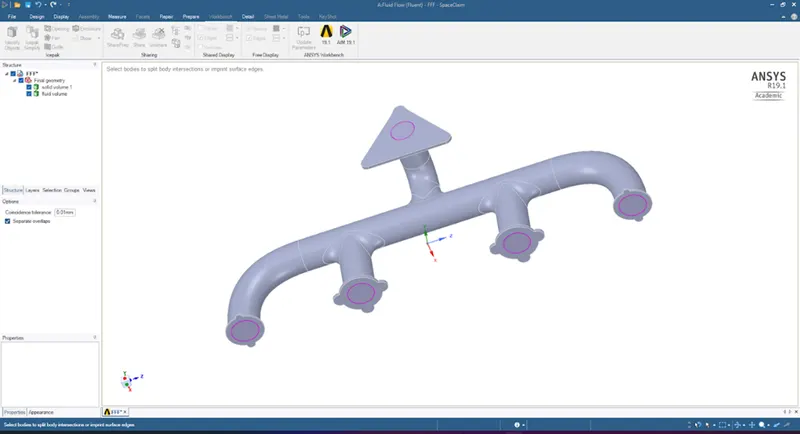
- Shareprep - Most important to do this step in geometry. If it is not done, then there'll be no interfaces where information is shared and mesh will definitely fail. Basically, this step takes care of creating interfaces.
Baseline mesh:
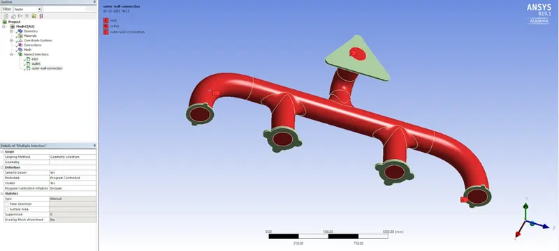
- Generally, it is always good to name the surfaces before meshing.
- select the edge you want to name by using edge selection -> then press N -> to name the selection.
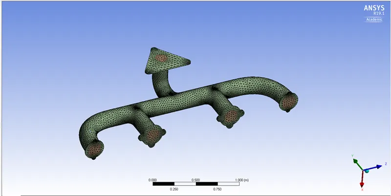
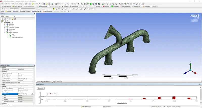
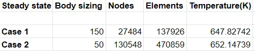
- Mesh size of 150 mm as default value.
- No. of nodes of 27484.
- No of elements of 137926.
Conformal mesh - There would be a face that both solid mesh and fluid mesh will share, which is perfectly interfacing or conforming to the solid mesh.
Non-conformal mesh- Actually there'll be a physical gap between two bodies, one vertex should connect with another vertex (not overlapped properly). In order to to do that, do share topology in geometry.
Inflation:
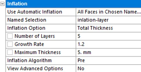
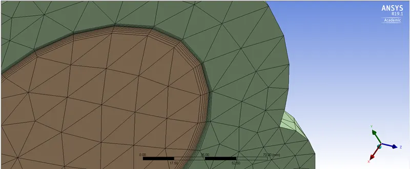
- Inflation layer helps us to create a body-fitted mesh. It means it creates a layer of mesh same as the geometry.
Mesh quality criteria:
Named selection (Initial condition):
Solution setup
Physics setup:
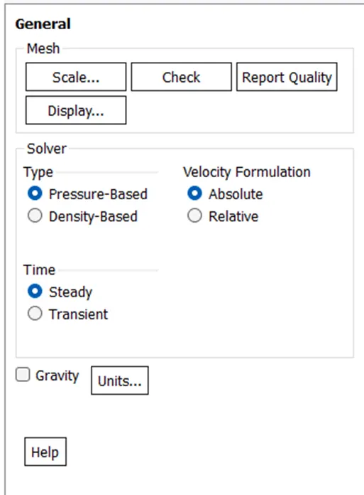
- It is a pressure-based solver type of steady state time to solve the problem and get results.
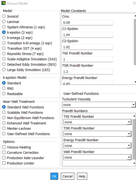
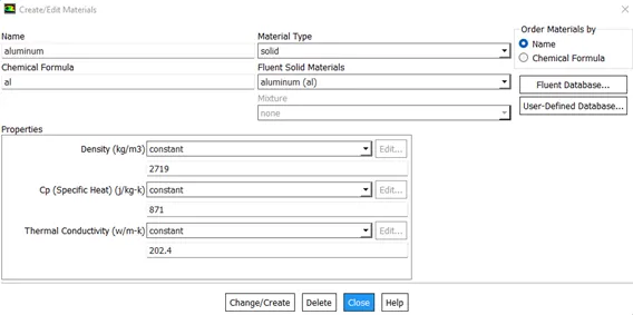
- As it has a high Reynolds number so will go to a k-epsilon model which is a turbulent model and contains temperature to predict conjugating heat transfer in this simulation.
Boundary conditions:
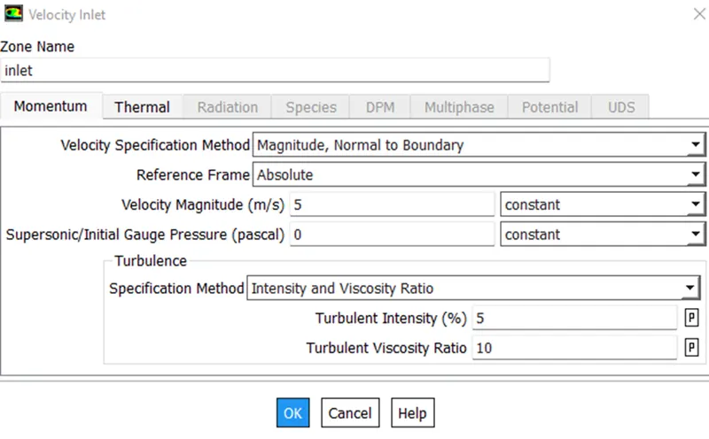
- Inlet: Inlet velocity of about 5 m/s and temperature of 700 kelvin(K).
-
Outlet: Pressure outlet: gauge pressure of 0 pa.
-
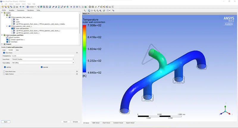
Outer wall convection: Thermal conditions => convection: Heat transfer coefficient = 20 W/m^2 K.
-
Flanges or Support: Thermal conditions =>Heat flux = 0 W/m^2 (Adiabatic walls).
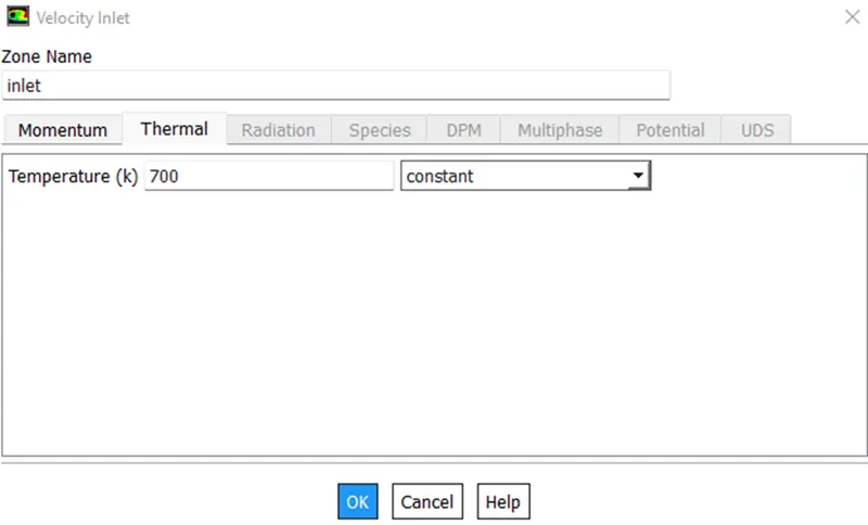
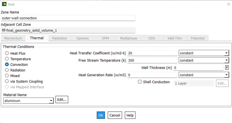
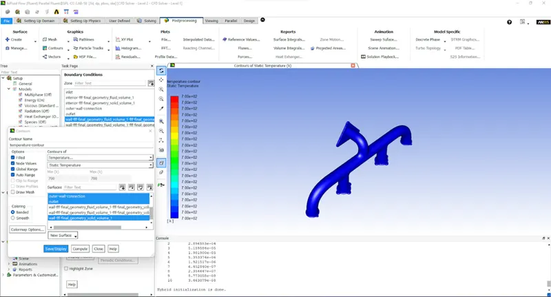
The initial contour of temperature:
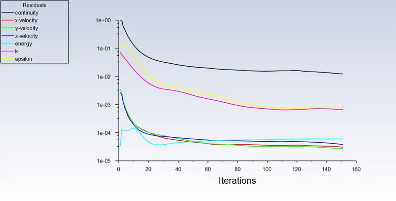
Scaled residual plots:
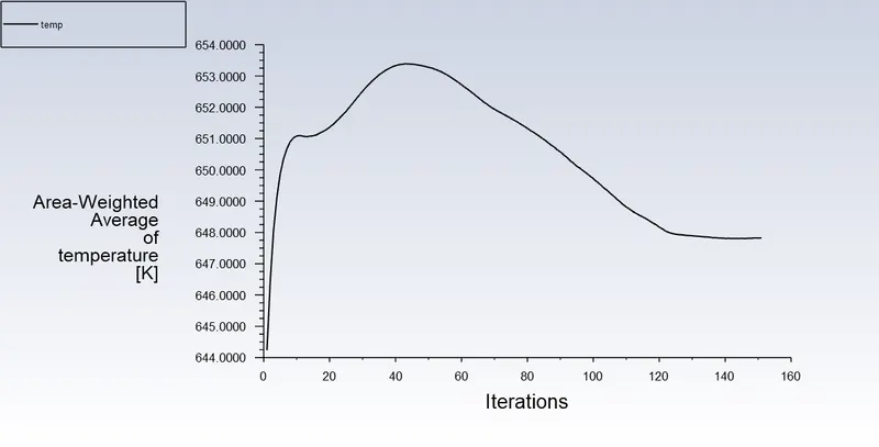
Temperature:
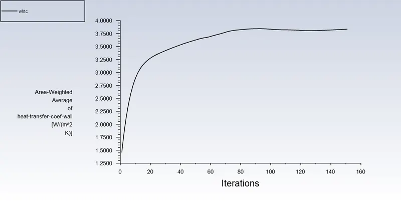
Wall Heat Transfer Coefficient:
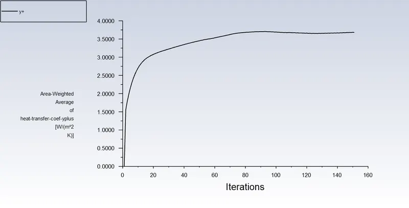
Yplus Heat Transfer Coefficient:
Post processor
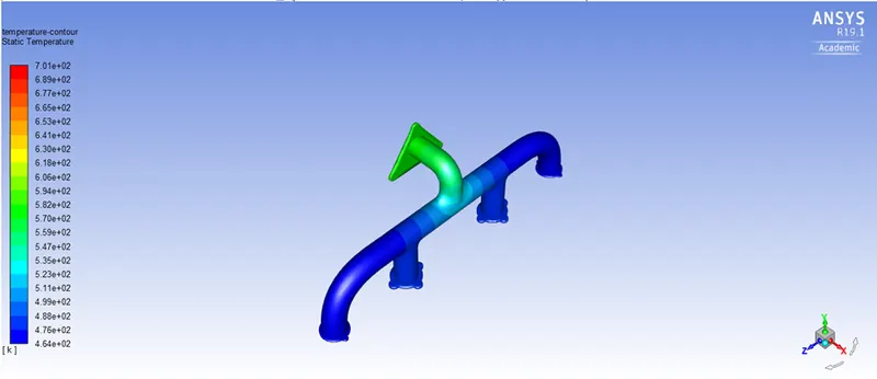
Temperature contour:
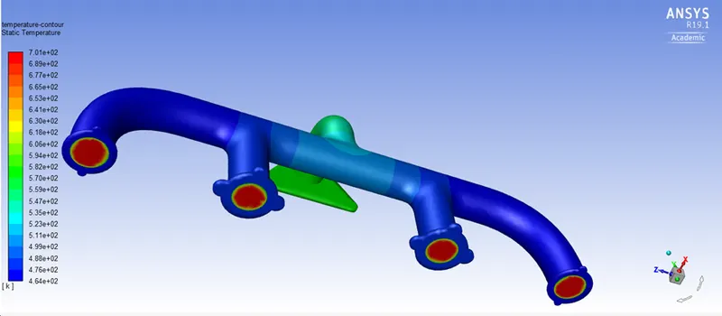
Temperature outer wall convection:
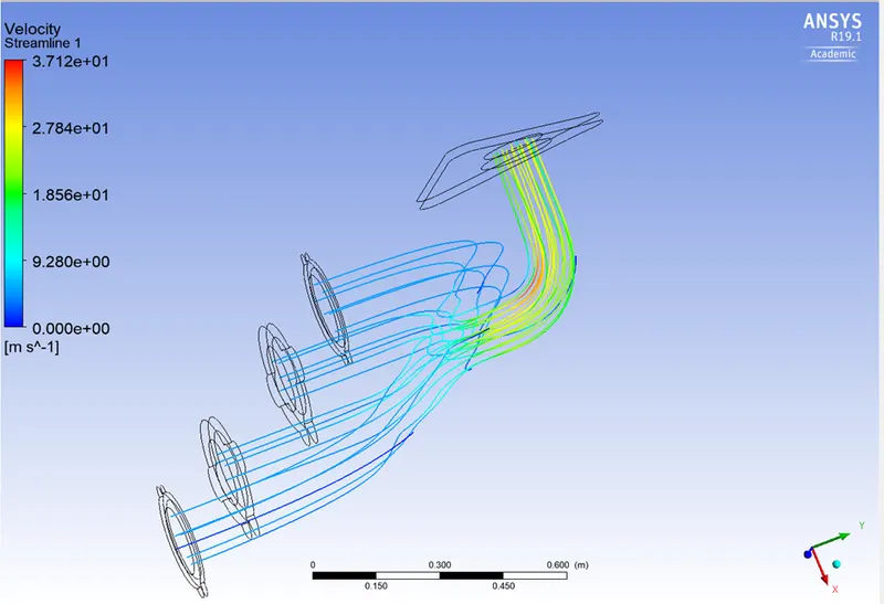
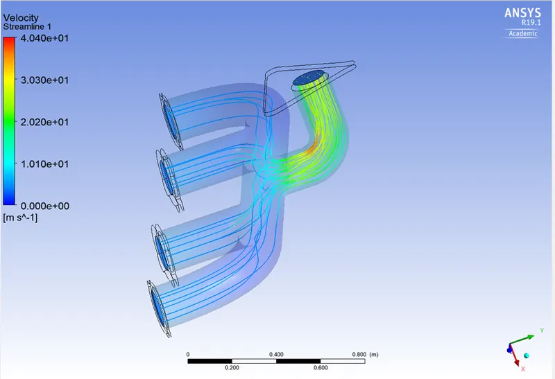
Velocity streamline:
Wall Heat Transfer Coefficient:
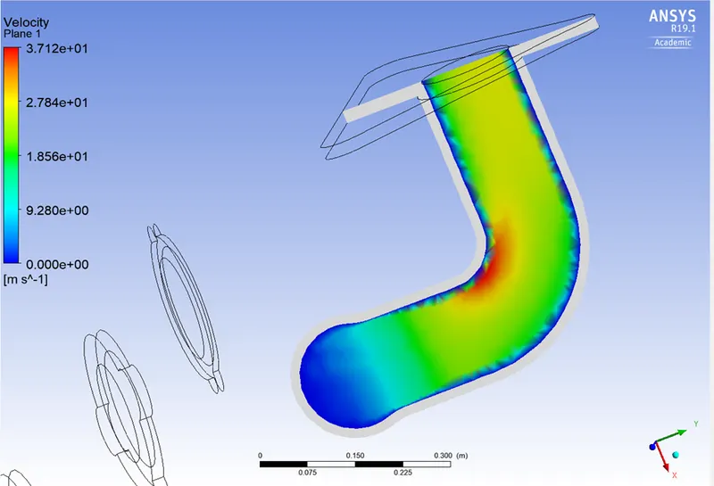
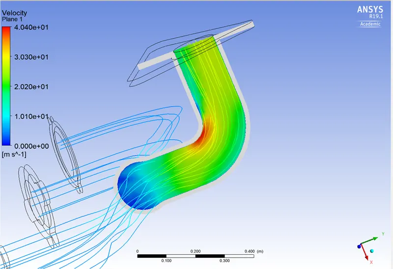
Velocity contour:
Case 2- Refined setup:
Simulating the flow with the Steady case 2:
Pre-processor
Meshing:
- Mesh size of 150 mm.
- No. of nodes of 130548.
- No of elements of 470859.
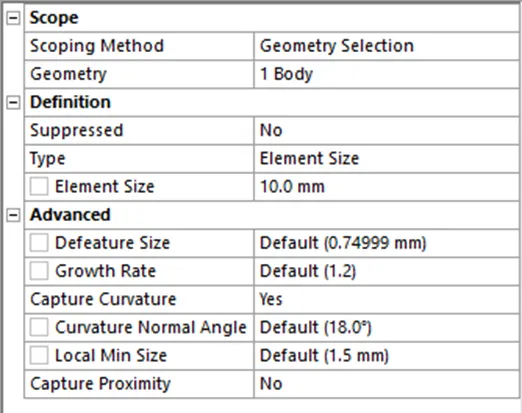
- Body sizing of about 10 mm.
Body sizing:
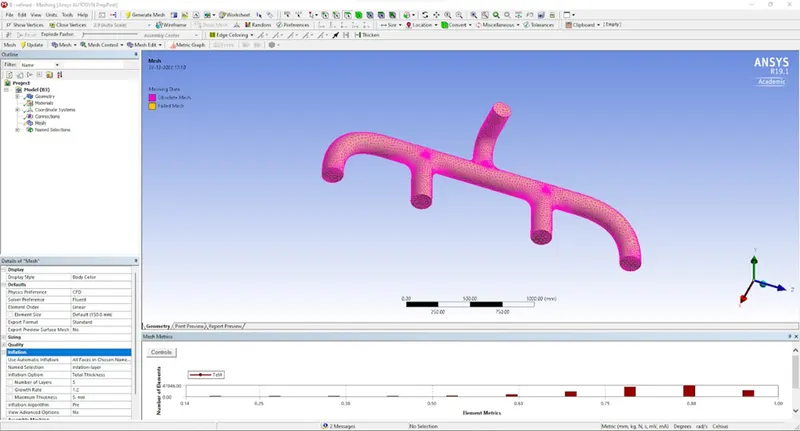
Inflation:
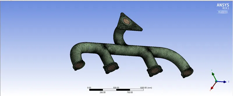
Fined mesh:
Solution setup:
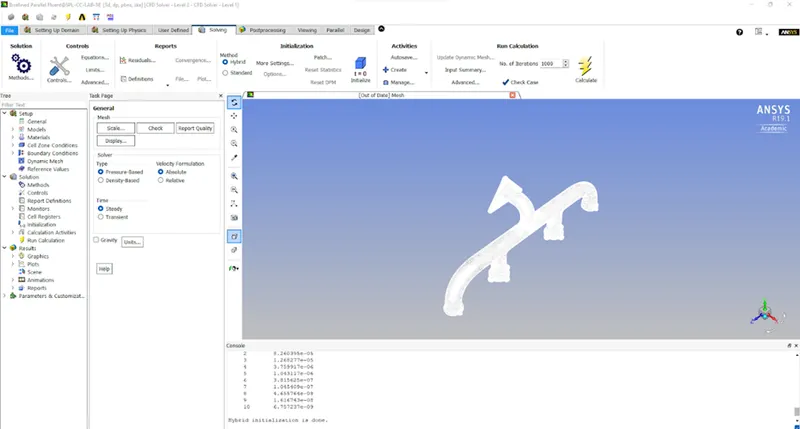
Scaled residuals plot:
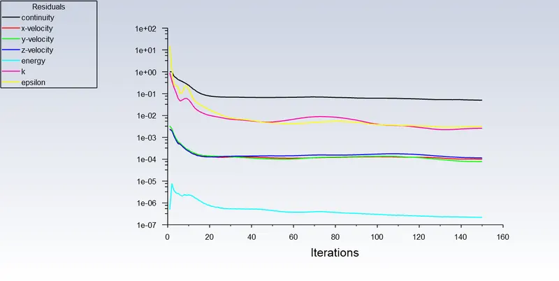
Temperature:
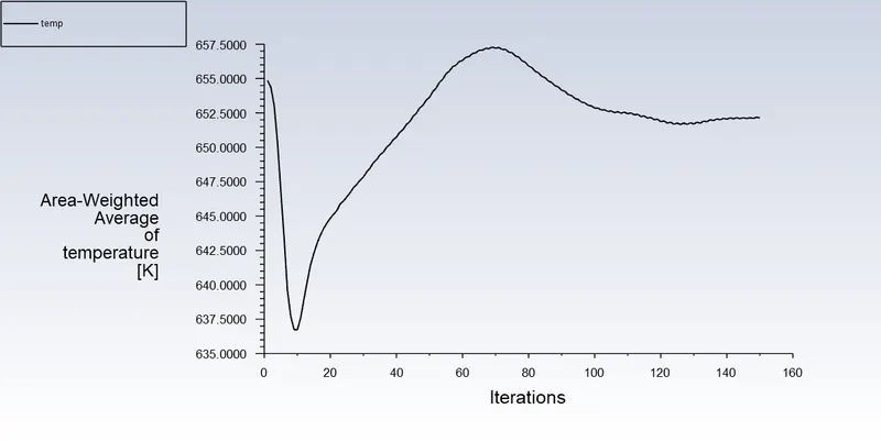
Wall Heat Transfer Coefficient:
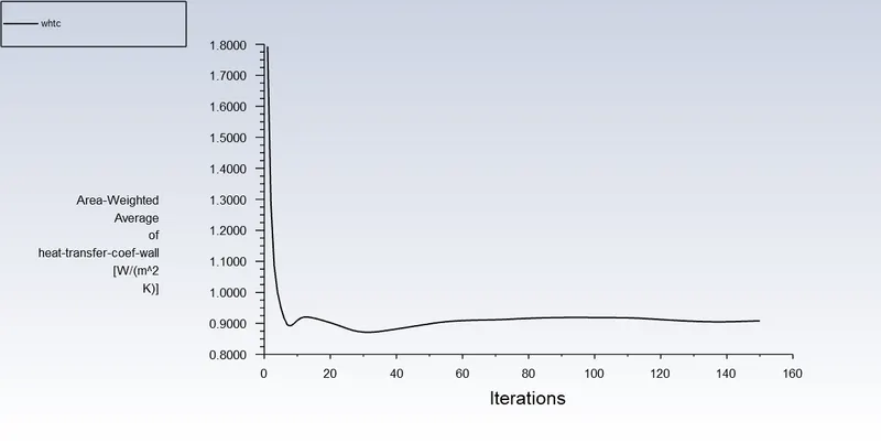
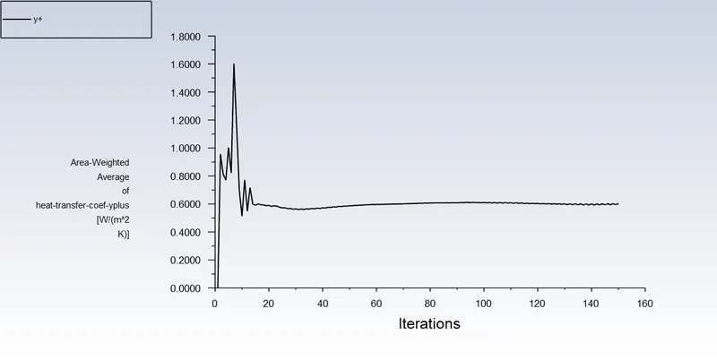
Yplus Heat Transfer Coefficient:
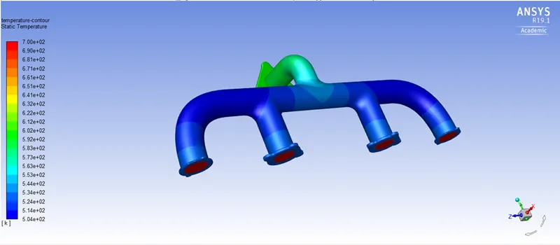
Static Temperature contour:
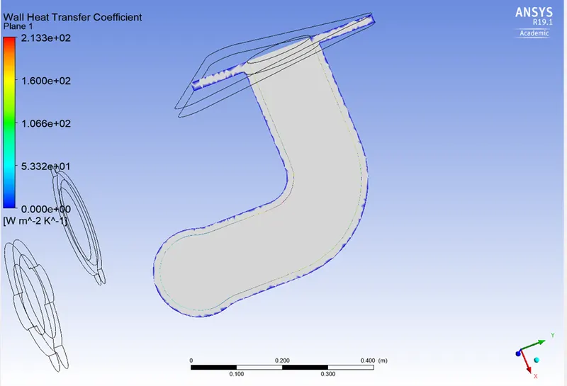
Wall Heat Transfer Coefficient:
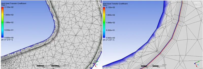
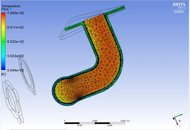
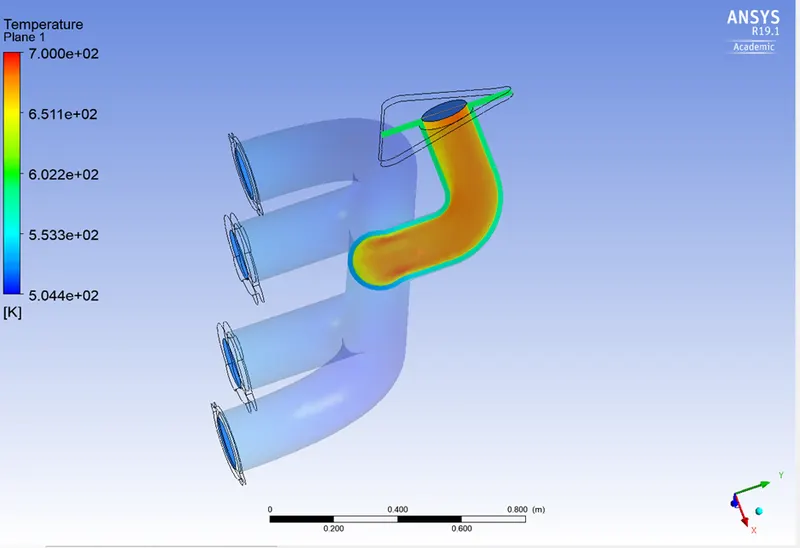
Temperature contour:
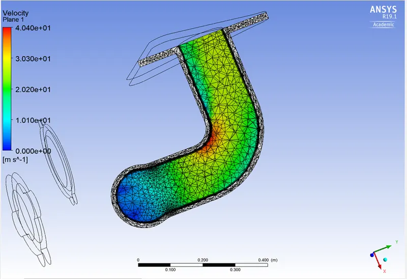
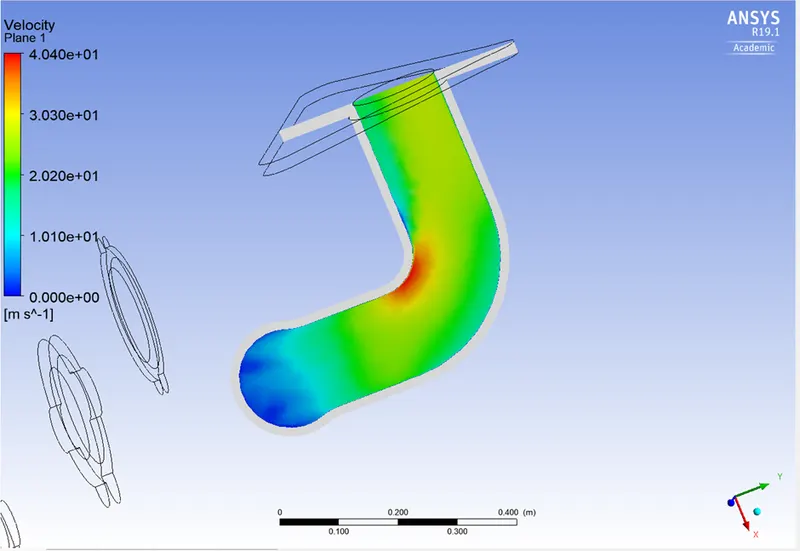
Velocity contour:
Velocity streamline contour:
Grid independence test:
Verifying the HTC(Heat Transfer Coefficient) predictions from the simulations :
- The Nusselt number is the ratio of convective to conductive heat transfer across a boundary.

- where h is the convective heat transfer coefficient of the flow, L is the characteristic length, k is the thermal conductivity of the fluid.
- Then this Nusselt number is related to the Reynolds number i.e.,

- Where,

and u is the flow speed (m/s)
- So if you observe heat transfer coefficinet is directly proportional to the Reynolds number (also to the velocity). So if you increase the velocity then there will be increase in the convective heat transfer coefficient. That's what we have proved above and if you want you can run another simulation by increasing the reynolds number of the flow then you will observe there will be increase in the overall convective heat transfer coefficient or at a particular location than in the previous low reynolds number simulation.
Factors that the accuracy of the prediction depends on :
- Mesh quality greatly impacts the accuracy of predicted value from our simulations which can be observed from the above contours and maximum values of related parameters like velocity and heat transfer coefficient.
- Appropriate y+ value helps in calculating total layer thickness from the wall for the better capturing of effects near walls, which is HTC in our case.
- An appropriate turbulence model has to be used in accordance with the y+ value which is very important.
- Appropriate solvers are one of the most important factors which lead all the calculations in solving the equations
- Inflation layers and boundary conditions.
Animated file link: