Week 4 - CHT Analysis on Exhaust port
Aim:
To run a simulation to analyze Conjugate Heat transfer in the Exhaust port.
Objective:
1. To understand why and where a CHT analysis is used.
2. Run the CHT simulation using different turbulence models and justify the results.
Introduction:
Conjugate Heat Transfer (CHT):
- The Conjugate Heat Transfer (CHT) analysis type allows for the simulation of heat transfer between solid and fluid domains by exchanging thermal energy at the interfaces between them. Heat transfer in a solid is called conduction and heat transfer in a fluid is called convection.
- Conduction occurs due to direct molecular collision. The faster kinetic energy collides with the low-speed kinetic energy and heat transfer occurs.
- The convection process is not happening alone. It is combined with conduction or radiation. (CONDUCTION + ADVECTION=CONVECTION).
- So, the Conjugate heat transfer occurred mostly in the cooling process like HEAT SINK, BATTERY COOLING, and AIRFLOW OVER THE SOLID OBJECT FOR COOLING.
- Whenever the solid and fluid interface appears, this type of CHT analysis can be done to find the optimum result by using Ansys. It allows the simulation of the heat transfer between solid and fluid domains by exchanging the thermal energy at the interface between them.
Conjugate Heat Transfer (CHT) Applications:
- Internal combustion engine
- Cross Flow heat temperature,
- Integrated Circuit Chips,
- HVAC
- turbocharger,
- Cooling of Electronic Devices, Burners, and Combuster
Why CHT analysis?
- Conjugate heat transfer (CHT) analysis can accurately predict heat transfer by simultaneously solving all the relevant solid and fluid flow field heat transfer processes, for example, conduction through solids, free and forced convection in the gases/fluids, and thermal radiation.
- In that wall heat transfer coefficients and their local variations on surfaces are directly calculated within the model rather than based on simplified empirical calculations.
- The CHT approach, therefore, has benefits for those applications where heat transfer is either non-uniform or difficult to calculate empirically.
Solving and modeling approach:
Geometry:
- Load the CAD model of the Exhaust manifold in Spaceclaim and check for any extra edges, remove them if any.
- Now volume extraction tool is used which is the process of extracting the fluid volume from the solid volume:. Go to Repair > Volume extract, and select the edges to separate the inner and outer volumes. Name the outer volume as Solid volume and the inner as Fluid volume and move both the volume to a new component and delete empty components.
- After this Share tool is used for sharing information from fluid volume to solid volume. It plays important criteria in CHT analysis: Go to workbench > Shareprep, to share the physics between the fluid and solid volume and conformal mesh can be achieved. Pink circles are seen after completing the process.
Meshing:
- Start the mesh section.
- Name the boundaries, which are Inlet, Outlet, Symmetry, Wall, and Car-wall.
- Then, provide a specific element size and generate the mesh.
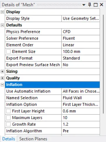
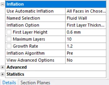
- Finally, add inflation layers according to correct y+ values. This completes the Mesh section.
Setup :
- First, we need to check the mesh from the Domain section.
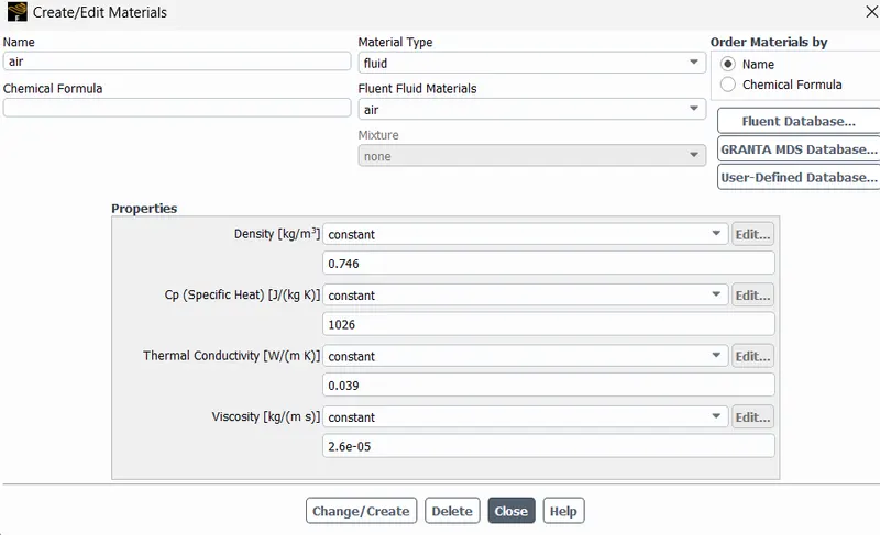
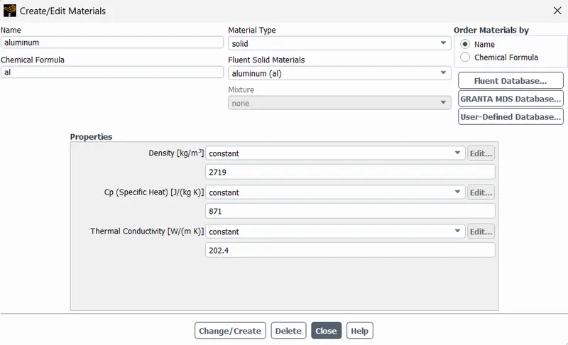
- Secondly, assign the materials and then check if the boundaries have been specified correctly.
- Now, provide the reference values according to the problem.
- Then, turn on the energy equation option, also set the turbulence model.
- Select the solver according to the problem.
- Now, set in the boundary conditions like inlet velocity, gauge pressure, etc.
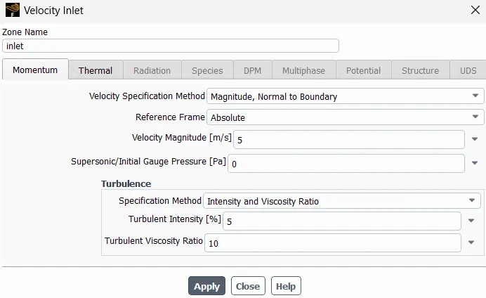
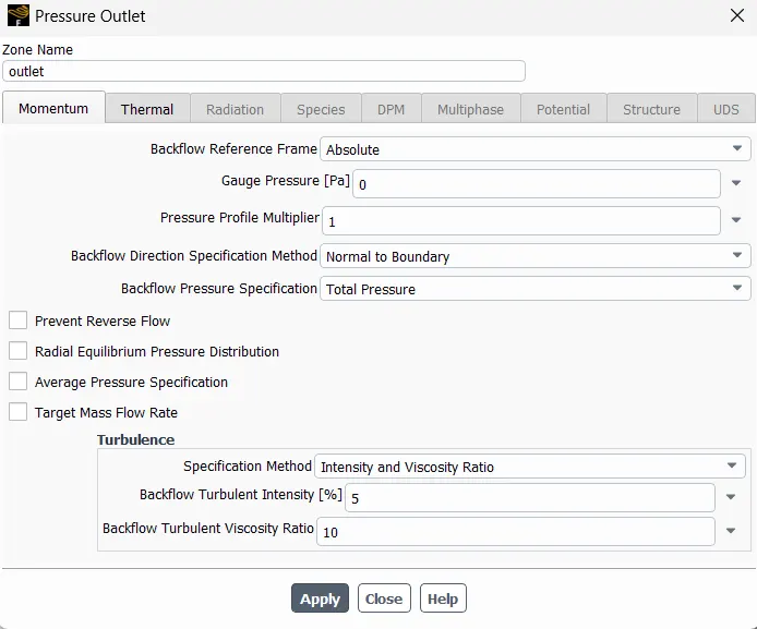
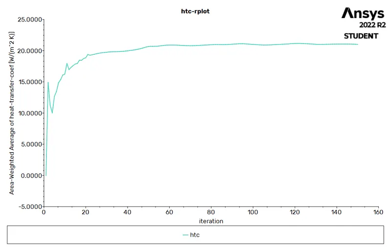
- In solution, creates HTC Report and also set the solution method.
- Initialize the problem with Hybrid Initialization.
- Go back to the result in the section and add velocity and pressure contours along a plane.
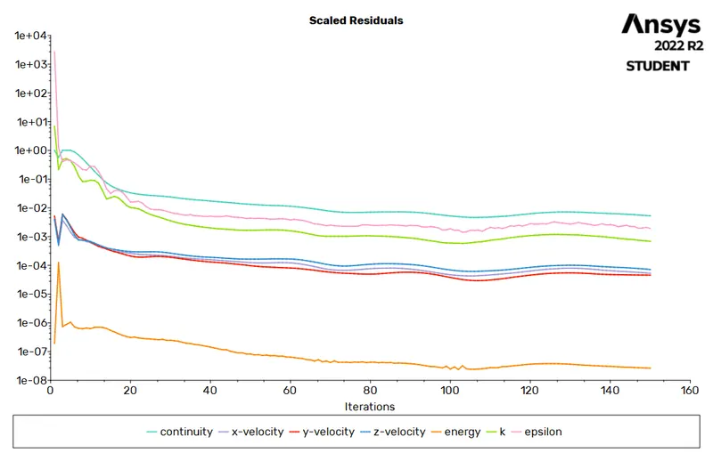
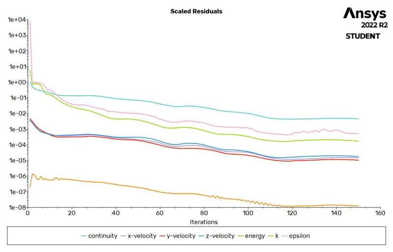
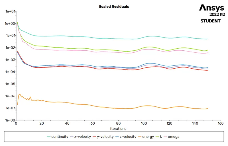
- Finally simulate the problem for some amount of iteration and observe the HTC and Residual plots.
- This completes the setup section.
Results :
- Select the wall volume to make it visible. Also, color it with the variable needed to be observed.
- After that, insert the plane and color it with variables like Pressure and Velocity which shows the Pressure and Velocity flow on the plane.
- Edit the legend according to requirement. This completes the results and hence the entire simulation.
Note: We will be performing 4 cases for different turbulent models.(k-epsilon: Standard, K-epsilon: Realizable, K- omega: Standard, K- omega: SST)
Case 1:
Mesh Size: 100 mm
Solver: K-epsilon standard
Mesh:
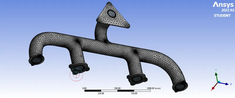
Residue Plot:
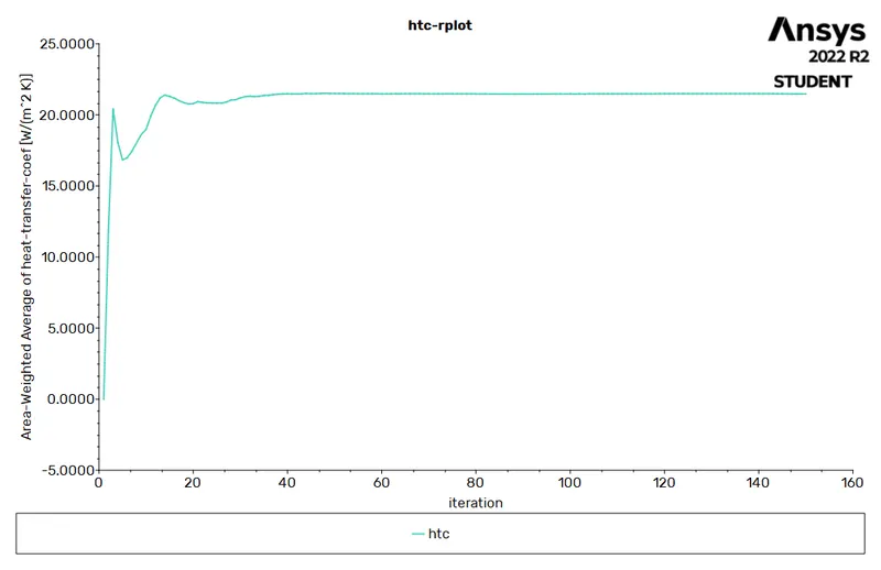
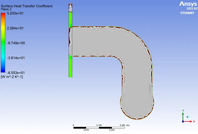
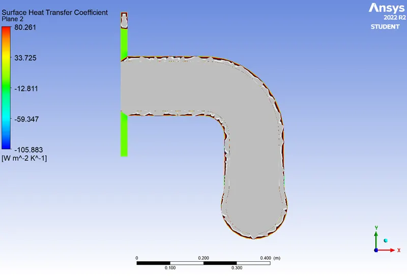
Surface Heat Transfer Plot:
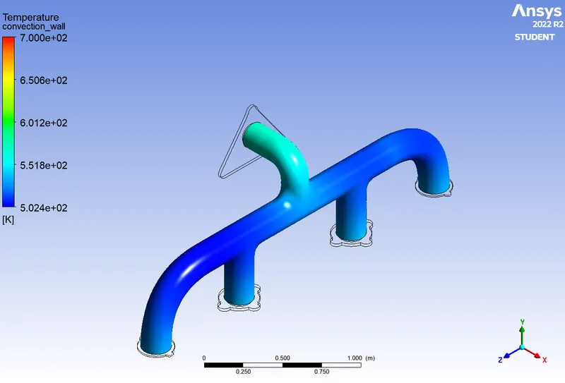
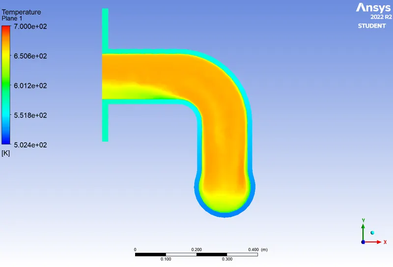
Temperature Contour:
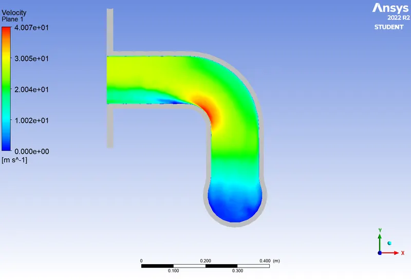
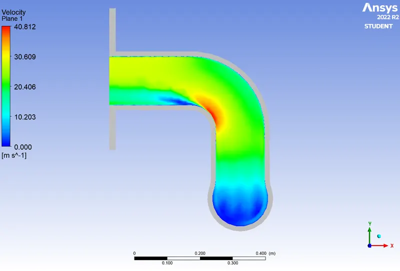
Velocity Contour:
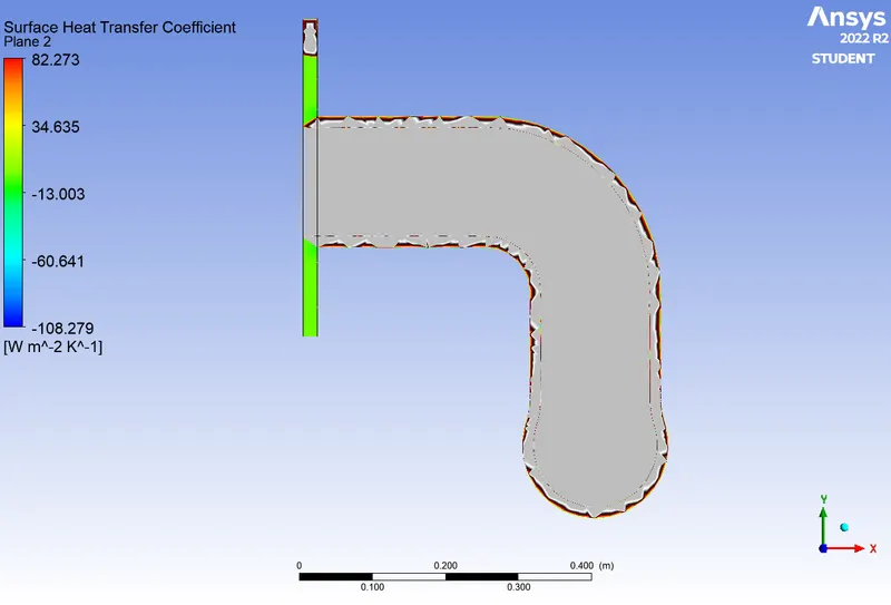
Wall Heat transfer coefficient:
Case 2:
Mesh Size: 100 mm
Solver: K-epsilon Realizable
Mesh:
Residue Plot:
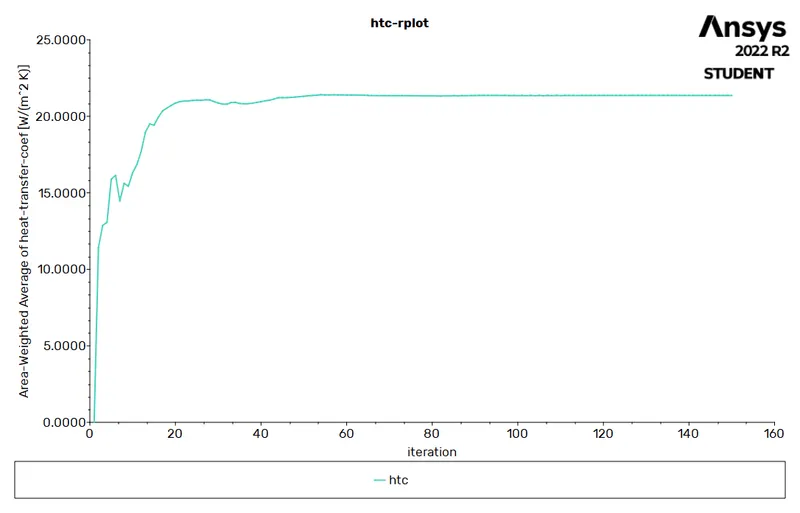
Surface Heat Transfer Plot:
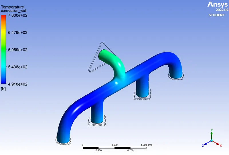
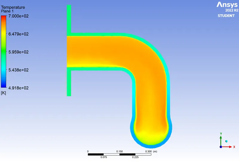
Temperature Contour:
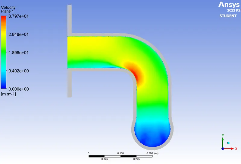
Velocity Contour:
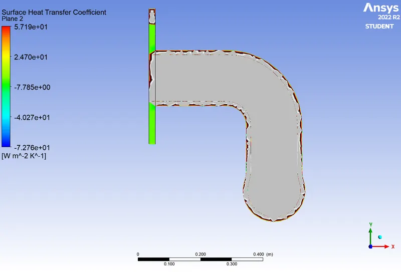
Wall Heat transfer coefficient:
Case 3:
Mesh Size: 100 mm
Solver: K- omega Standard
Mesh:
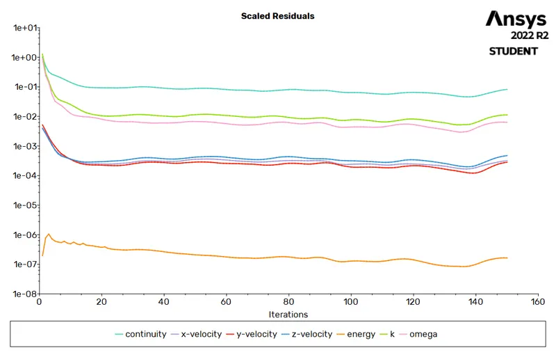
Residue Plot:
Surface Heat Transfer Plot:
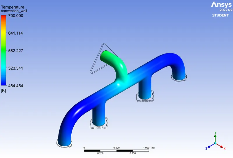
Temperature Contour:
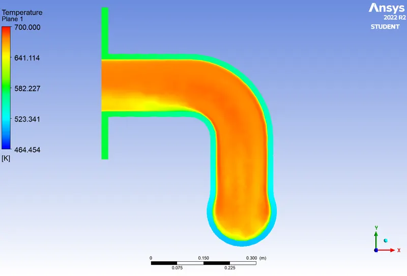
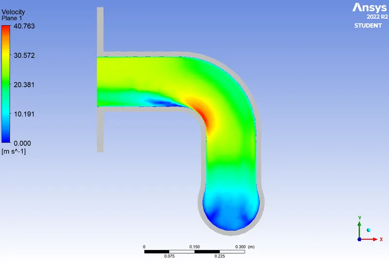
Velocity Contour:
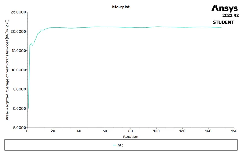
Wall Heat transfer coefficient:
Case 4:
Mesh Size: 100 mm
Solver: K- omega SST
Mesh:
Residue Plot:
Surface Heat Transfer Plot:
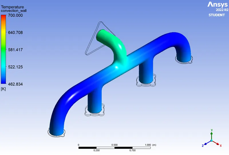
Temperature Contour:
Velocity Contour:
Wall Heat transfer coefficient:
Inferences:
The Wall heat transfer coefficient from the different viscous model is tabulated as follow:
| Sr. No. | Viscous Model | Wall Heat Transfer Coefficient |
| 1 | K-epsilon standard | 21.4723 |
| 2 | K-epsilon Realizable | 21.3621 |
| 3 | K- omega Standard | 20.9859 |
| 4 | K- omega SST | 21.00753 |
- No difference in Temperature contours for all three viscous models is observed.
- The maximum heat transfer coefficient is found at the layer adjacent to where the maximum velocity is found.
- Maximum wall heat transfer is found using K-epsilon standard viscous model.
Verify HTC :
Under forced convection circumstances, we can determine the heat transfer coefficient by using the Dittus-Boelter
correlation. Using the Dittus-Boelter correlation the heat transfer coefficient can be calculated in the following way using
two further dimensionless groups, the Reynolds number and the Prandtl number:
h = (k/D )*Nu
where k is the thermal conductivity of the liquid, D is the Hydraulic diameter, and Nu is the Nusselt Number which is
determined by the following equation:
Nu = 0.023Re Pr^n
where, n= 0.4 when fluid is being heated
n= 0.3 when fluid is being cooled
the Nusselt number is calculated as Nu = 131.792
In this equation, Re is the Reynolds number which equates to:
Re = (m D )/(μ)
The Reynolds number of the flow is Re = 56867.66 considering the flow velocity = 5 m/sec
and Pr is the Prandtl number :
Pr = (CP* μ)/k
the Prandtl number is Pr = 0.744
For the Reynolds number, m is equal to the mass flow rate. For the Prandtl number, CP is equal to heat capacity, and in both
equations, μ is the viscosity of the fluid in consideration. Once we have all of these factors, we can get a decent
estimation of the heat transfer. Also, we can get the estimation from some published papers or from some experimental values.
Here we find the theoretical value and the computational value of the surface heat transfer coefficient to be = 19.52 w/m^2k.
Accuracy of HTC prediction :
The accuracy of the predictions depends on several things,
- Accurate geometry of the model.
- It's Mesh quality.
- Inflation layers.
- Properties of material being used.
- Turbulence models.
Conclusion :
1. Here we find the theoretical value and the computational value of the thermal specific heat transfer coefficient to be = 19.52 so the value is really close to the value of h in the computational way which is = 20 w/m^2k.
2. Two factors influence the performance simultaneously: (a) Flow is developing along the length and the heat transfer coefficients tend to decrease along flow (b) Turbulence;
3. At the same time, turbulence is developing with tube rows at the bent, which would increase heat transfer coefficients.
4. The maximum heat transfer results at the bend of the exit port, It is because to ensure the conservation of mass at the exit port velocity should be more, which results in higher velocity and increase in velocity to attain a Reynolds number that is sufficient to make flow turbulent and higher Nusselt number at pipe bent at the exit, which increases Heat transfer co-efficient at that location.