Week 4 - CHT Analysis on Exhaust port
CHT Analysis on Exhaust port
Conjugate Heat Transfer (CHT)
The Conjugate Heat Transfer (CHT) analysis type allows for the simulation of heat transfer between solid and fluid domains by exchanging thermal energy at the interfaces between them. Typical applications of this analysis type exist as, but are not limited to, the simulation of heat exchangers, cooling of electronic equipment, and general-purpose cooling and heating systems.
In an IC engine simulation the accuracy very much dependent on how closely the system is modelled to mimic the natural system. Since the metal parts in the engine will be interacting thermally with the fluid domain a specified temperature profile may not be maintained throughout usually. The best method to replicate actual scenario will be considering walls also for the simulation.
In Urea/SCR after treatment system the key challenge is to Predict and mitigate the urea deposit formation. The sprayed urea-water will be impinging on the walls as a liquid film. The decomposition of urea and the formation of undesirable deposits are highly dependent on wall temperature, and the heat transfer between the film and the wall is important to capture. Predicting the wall temperature helps you identify areas that are vulnerable to wall deposition.
In the electro mobility system high powered motors will be working which will be having a huge power density which requires dedicated cooling system. The under prediction of heat load will cause the reduced cooling and hence the demagnetization may be happening for the permanent magnets.
Resolving the spatially varying surface temperature distributions in pumps and compressors improves the accuracy of the simulation and provides useful temperature data. For example, in a twin screw compressor, thermal expansion affects the clearance between the rotors. If that effect is not captured then the simulations will incorrectly predict leakage flows and lower the accuracy of the results.
CHT ANALYSIS ON A MODEL OF AN EXHAUST PORT
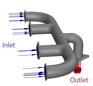
Here we use the inline four-cylinder engine exhaust manifold. where the conjugate heat transfer is analyzed to find the optimum heat transfer coefficient. Fluid volume is extracted from the port and consider as the fluid region where the air enters into the region. Since it has the interface of the solid and fluid domain so this type is called as CHT analysis. When we generate the baseline mesh. the non-conformal mesh is generated which affect the result To make a Conformal mesh Share topology option is used which make the perfect mesh.
SETUP:
Pressure based solver is used for this analysis. Steady state and enable the energy to measure the temperature. The turbulent k-epsilon method is used to run the analysis.
BOUNDARY CONDITION:
Material- air.
Inlet- velocity Inlet- 5m/s.
Temperature-700k
The outer wall of the port - convection. Heat Transfer coefficient-20w/m^2k.
Free stream Temperature-300 k
Viscous Model : k-epsilon.
Outlet- Pressure outlet.
Geometry
Case 1 : Baseline simulation
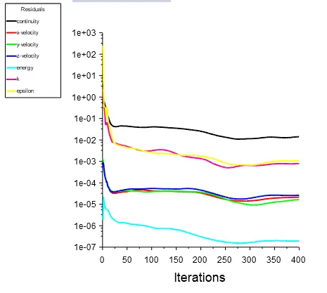
A Base line case has been made and simulated the flow and heat transfer phenomenon. The baseline mesh was having 136030 elements on it with a maximum skewness of 0.81435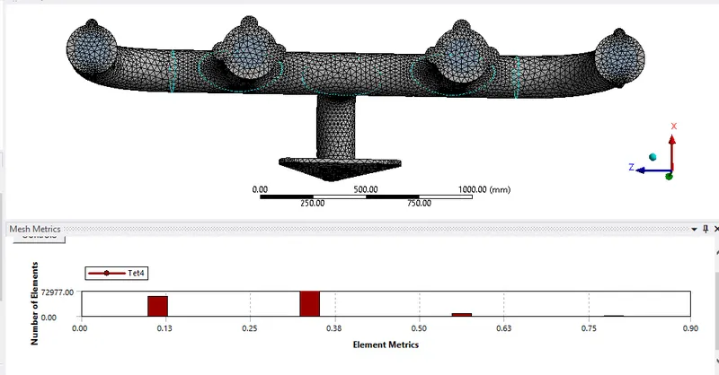
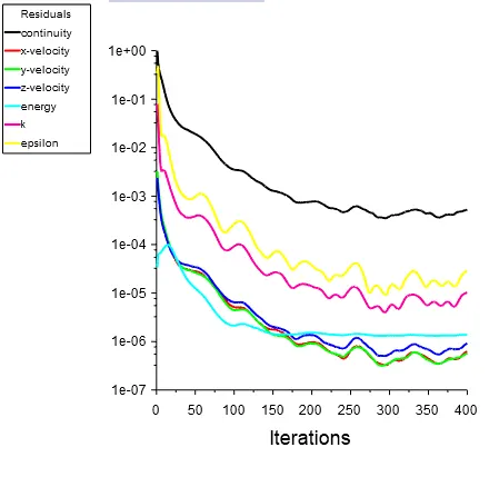
Residual plots
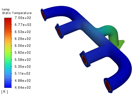
Temperature contour
Velocity streamlines
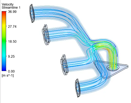
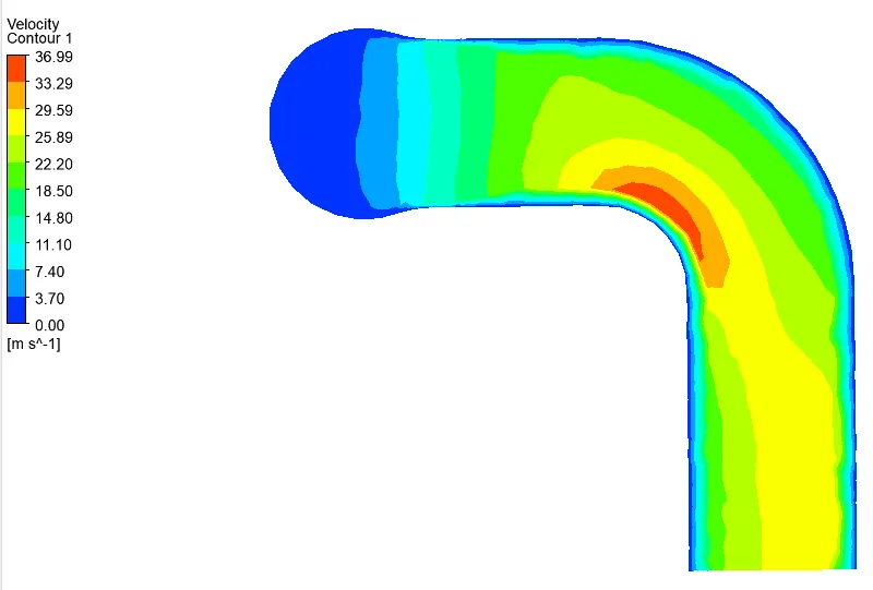
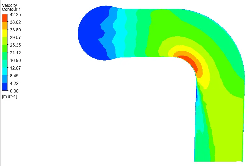
Velocity contour at outlet throat
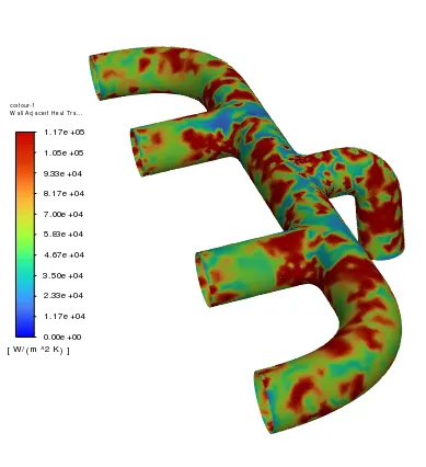
Wall heat transfer coeffiecent.
Case 2 : Refined simulation
Mesh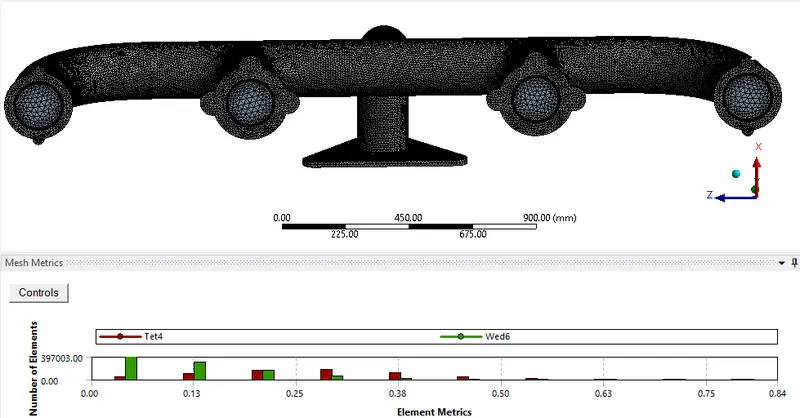
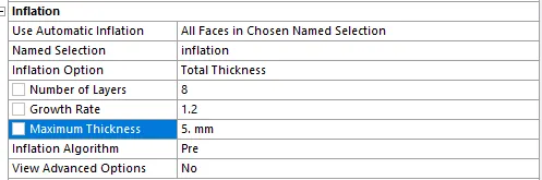
The maximum skewness observed was 0.8364 and the total mesh count was 1553521. The avarage Solution is set up with SST K omega model. The current inflation layer settings will give a y+ around 5 which will be a best fit in it's range (1 - 10)
Residual plots
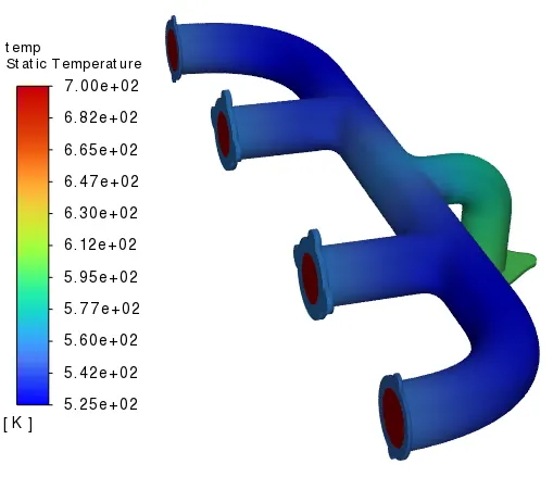
Temperature contour
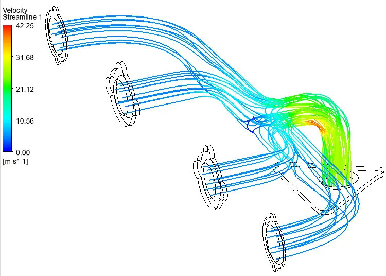
Velocity streamlines
Velocity contour at outlet throat
Wall heat transfer coeffiecent.
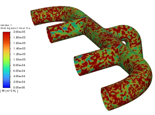
| Sl No. | No. of Element | Wall HT Coefficient
[W/(m^2 K)] |
| Case 1 | 136030 |
21.19 |
| Case 2 | 1553521 |
21.33 |
Verification of results and factors affects the accuracy of the prediction
According to Bernoulli's mass conservation principle mass is conserved in our model which is clearly explained below;
Let us assume the flow rate from each inlet as Q1, Q2, Q3, Q4 respectively, and Q5 be the flow rate from the exhaust manifold.
As mass is neither created nor destroyed, mass flow rates are also balanced as below;
`Q1+Q2+Q3+Q4=Q5`------(1)
we have `Q= rho*A*V` ------(2)
Now equation 1 becomes
A1V1+A2V2+A3V3+A4V4=A5*V5
As it is an incompressible flow to compensate for mass flow, velocity is increased. and the overall mass flow rate is conserved. As velocities are high, the Reynolds number at the outlet manifold will be high.
`Nu=f(Re,Pr)` for forced convection application.
`Nu= (hD)/k`
from above formula `Nu ∝ Re` .
Hence `Nu∝h`.
therefore, `Re∝h`.
From our simulation, we have observed velocities are high at bend section of outlet manifold hence higher Reynolds number which was at high heat transfer coefficient. Therefore predictions from our simulations can be considered correct.
Factors that influence accuracy of predictions:
- Mesh quality greatly impacts the accuracy of prediction value in our simulations which can be observed from above contours and maximum values of related parameters like velocity and heat transfer coefficient.
- An appropriate turbulence model has to be used in accordance with the y+ value which is very important.
- Appropriate y+ value helps in calculating total layer thickness from the wall for the better capturing of effects near wall, which is Heat transfer coefficient in our case.
References: