Week 4 - CHT Analysis on Exhaust port

AIM -

A steady-state simulation is to be performed to study Conjugate Heat Transfer (CHT) Analysis on the Exhaust Port model in Ansys Fluent.

INTRODUCTION & THEORY -

1) Conjugate Heat Transfer (CHT) can be defined as the heat transfer between solid and fluid domains by exchanging thermal energy at their interfaces. That is, it comprises both conduction & convection modes of heat transfer. Heat exchangers, the cooling of electronic devices, and cooling and heating systems are a few examples of the Conjugate Heat Transfer phenomenon.

2) An exhaust port may be defined as the opening, in the cylinder or valve, by which the air (exhaust steam) escapes.

3) Conduction is the mechanism of heat transfer in which energy exchange takes place from a region of high temperature to a region of lower temperature by the kinetic motion or direct impact of molecules and by the drift of electrons. The latter applies particularly to metals, which are both good electrical conductors and heat conductors. Essentially, conduction is heat transfer by molecular motion in solids or fluids at rest.

Fourier's law of heat conduction states that the rate of heat flow by conduction in a given direction is proportional to the area normal to the direction of heat flow and to the gradient of the temperature in that direction.

`Q_(cond) = - k A frac{dT}{dx}`

`Q_(cond)` is the rate of heat flow through area `A` in the positive x-direction. Heat will only flow in the positive x-direction if the temperature is decreasing in that direction, hence the negative sign, as `frac{dT}{dx}` must be negative for `Q_(cond)` to be positive i.e. heat flows “downhill”. The proportionality constant, `k` is called the thermal conductivity of the material. Good conductors have high values of `k`, and good insulators have low values. `k` has SI unit `W/(mK)` and varies from around 0.1 `W/(mK)` for gases and insulating materials to up to 1000 `W/(mK)` for highly conducting metals such as copper or silver. The thermal conductivity of a material can be defined as the rate of heat transfer through a unit thickness of material per unit area per unit temperature difference. It is a measure of the ability of a material to conduct heat a higher value for thermal conductivity indicates that the material is a good hit conductor and a low value indicates that the material is a poor heat conductor or a good insulator.

4) The process by which the transfer of heat occurs from one point to another within a medium due to the actual motion of the heated particles of the medium is known as Convection. Cooling of a room due to AC or warming up due to a radiator can be attributed to convection. It may be defined as a mode of energy transfer that involves the combined effects of conduction and the fluid motion between a solid surface and an adjacent moving liquid or gas. The faster the fluid motion, the higher the convective heat transfer.

5) Newton's law of Cooling states that the convective heat transfer is proportional to the difference in temperature between an object and its surrounding.

`Q_(conv) = hADeltaT`

where, `Q_(conv)` is Convective Heat Transfer,
`h` is Heat Transfer Coeffiecient,
`A` is Normal Surface Area,
`DeltaT` is Temperature Difference

6) Thermal Diffusivity (`alpha`) is a measure of the rate at which heat disperses throughout an object or body. Larger values of `alpha` will lead to faster heat dissipation in the material. The material with a higher value of `k` and a lower value of `rhoc`. A High value of `k` will result in faster energy transfer through the material. A low value of `c` means a lesser amount of heat moving through the material will be used for raising the temperature and more of it will be available for transfer. The unit of thermal diffusivity is `m^2/s`.

`alpha = k/(rhoc)`

7) Nusselt number (`N_(uL)`) is the ratio of convective heat transfer to conductivity transfer within a fluid region. It denotes the increasing heat transfer through a fluid layer caused by convection, relative to conduction. When fluid is motionless, conduction will be dominating mode of heat transfer (Nusselt number = 1). When there is a bulk fluid motion convection, it will be higher.

`N_(uL) = frac{h}{k / L} = (hL)/k`

8) Prandtl number (`Pr`) is the ratio of momentum diffusivity to thermal diffusivity. It compares the velocity boundary layer thickness to the thermal boundary layer thickness. Prandtl number for gasses is almost one. For water, it is in order of 10. It is 0.01 for liquid metals and 10 to power five for heavy oils. ()

`Pr = nu/alpha`

9) Y plus is a non-dimensional distance. It is the distance from the wall which is measured in terms of viscous length.

The fluid flow parameters at the fluid wall (boundary layer) were to be recorded for this analysis because both convection and conduction, two types of heat transfer, were involved. There could be four sections of layers at the boundary layer during fluid flow over any surface. A viscous sublayer is a very thin layer that is next to a wall where viscous effects predominate. Although flow is still mostly controlled by viscous effects, the turbulent effects appeared to be considered next to the viscous sublayer in the buffer layer. The overlap layer, also known as the log law layer, is above the buffer layer and has significantly more noticeable turbulence effects. Finally, there existed a layer of turbulent air where the turbulent effects dominated the viscous effects.

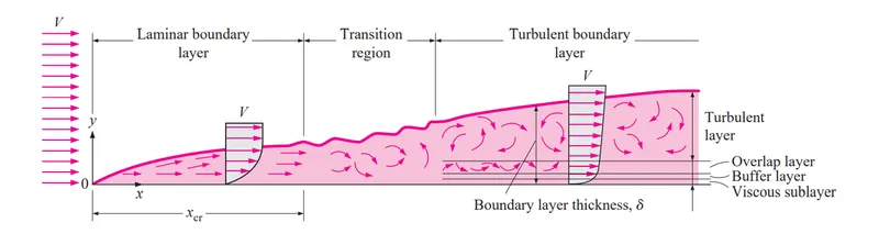As a result, since the analysis was of the "near wall" type and viscous effects were particularly prominent at the wall, a turbulence model with a low Reynolds number was meant to be selected for this situation as `Re = frac{rhoVx}{mu}`.

Among all the turbulence models the 'k omega SST' model is best suited for near-wall type analysis with a 'y plus' value ranging between 1 to 5. Thus, the k omega SST model was used for the simulation study.

SOLVING & MODELLING APPROACH -

The workflow for every CFD simulation is as follows:

1) Problem finding
2) Pre-processing
3) Processor or Solver
4) Post-processing

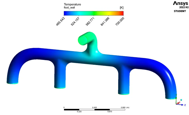
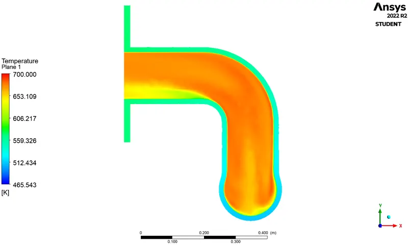
Three different types of heat transfer can be seen in the held model of the exhaust port: convection between the inner surface of the exhaust port and the fluid, conduction within the surface, and third, convection between the fluid and the outer surface wall. Four inlets with a temperature of 700 K and a velocity of 5 m/s allow fluid (air) to enter this exhaust port. There is a pressure outlet condition at the single outlet. While the internal solid surface's heat transfer coefficient needs to be determined and verified, the outer surface wall is given a 20 W/m²K heat transfer coefficient.

The temperature of the fluid (air) inside the exhaust port, `T = frac{T_i + T_o}{2} = frac{700 K+ 300 K}{2} = 500 K implies 200°C`

The imported exhaust port model underwent geometry simplification, including volume extraction, topology sharing, and mesh generation with inflation layers. After running the simulation with the necessary solver settings, the required result values were computed. The outcomes were derived in the post-processing stage, and from them, relevant inferences were made. Results were lastly verified using mathematical calculations.

PRE-PROCESSING -

The Exhaust Port model was imported followed by volume extraction using the 'Volume Extract' tool in Prepare Toolbar. Later, the 'Share' tool was used to allow the topology sharing of coincident surfaces.

Note: Do not suppress the outer surface (wall) of the model as there is a transfer between the outer wall and the fluid as well, which is an integral part of this simulation study.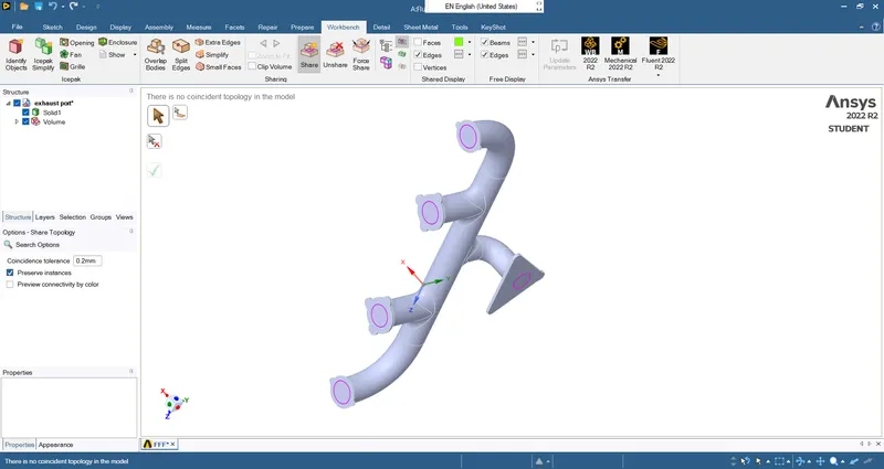



In the 'Mesh' file, name selection was accomplished before proceeding toward the mesh generation as;

1. Inlets (all four inlets)
2. Outlet
3. Convection Wall (outer wall )
4. Fluid Wall (wall inside the outer wall)
5. Fluid Domain (the entire domain in which fluid, that is, air will flow)

As all four inlets were asked for the same inlet conditions, a combined name selection was done. Otherwise, separate name selections could be assigned.



Mesh was generated using a finer baseline element size of 18 mm. Later, inflation layers were supposed to be created for the 'Fluid Domain' at the boundary of the 'Fluid Wall' so as to effectively capture the velocity gradient and parameters at this boundary.

For inflation layers, the value of the first layer thickness was calculated using an external calculator as:

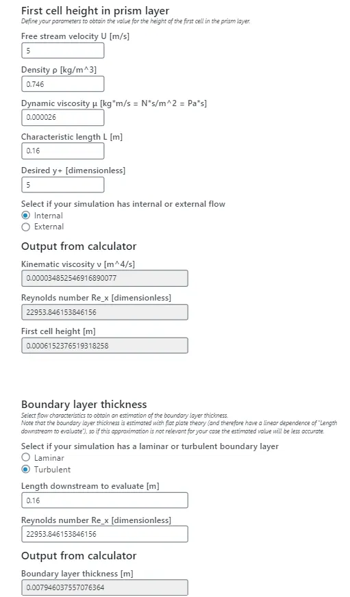
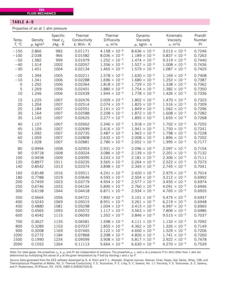
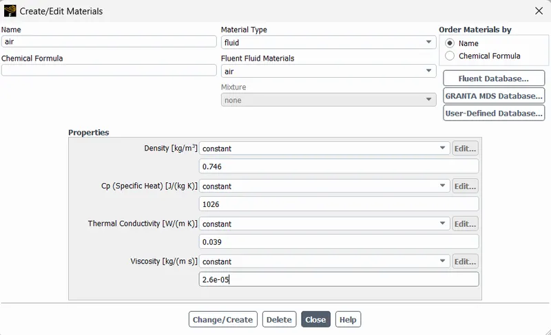
For air at 1 atm pressure and 200°C temperature, values were taken from a reference book as:

Thus, inflation layers were generated:

First Layer Height = 0.6 mm
Maximum Layers = 12
Growth Factor = 1.25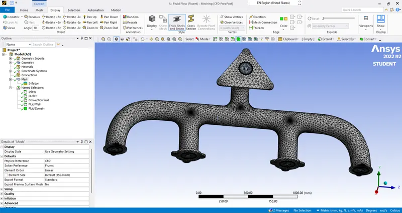




PROCESSING / SOLVER -

Fluent Setup
Sr. No.	Setup	Command
1	Solver Type	Pressure based
2	Solver Time	Steady State
3	Energy	ON
4	Turbulence Model	K omega SST
5	Material (Fluid)	Air (changing the properties of air 'at 200°C')
6	Inlet	Velocity Inlet (5 m/s); Temperature – 700 K
7	Outlet	Pressure Outlet
8	Outer (Convection) Wall	Wall – Convection – 20 W/m²K
9	Internal Solid Surface (Fluid Wall)	Wall BC
10	Method	Coupled

A report to calculate the heat transfer coefficient was prepared using the 'Report Definitions' tool.

After completion of the solver settings, the simulation was initialized and ran for a certain number of iterations. Even though the simulation didn't converge, observing the plots it was confirmed that the results have converged.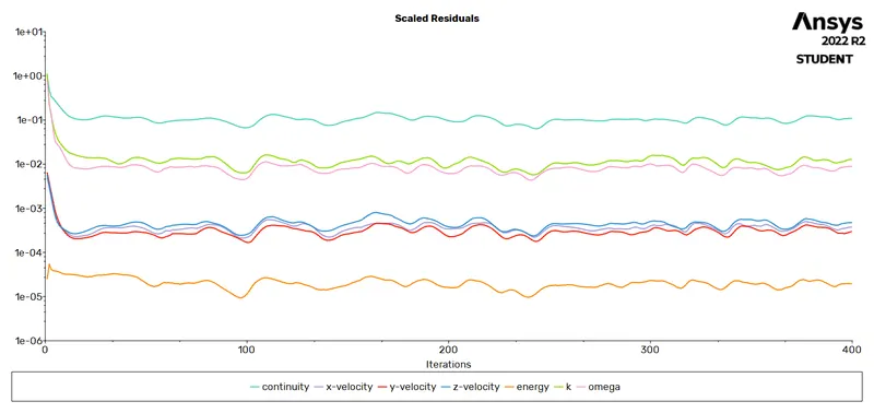

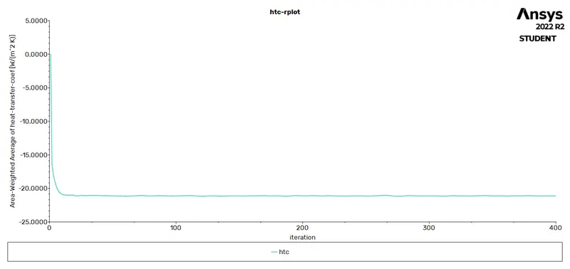
The value of the heat transfer coefficient computed for the internal surface (fluid wall) was found to be `21.12 W/(m^2K)`.

Note: The value of the heat transfer coefficient was computed by varying the element size during the mesh generation stage and it was observed that this value had no significant difference during each case. Thus, `21.12 W/(m^2K)` was considered as the final computed value through numerical computation.

POST-PROCESSING -

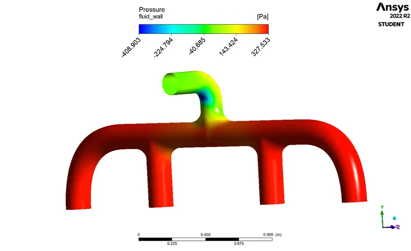
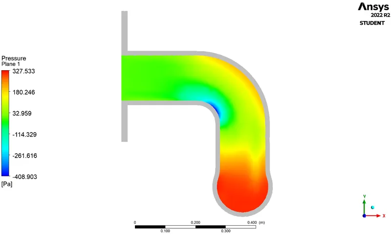
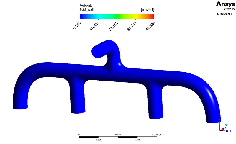
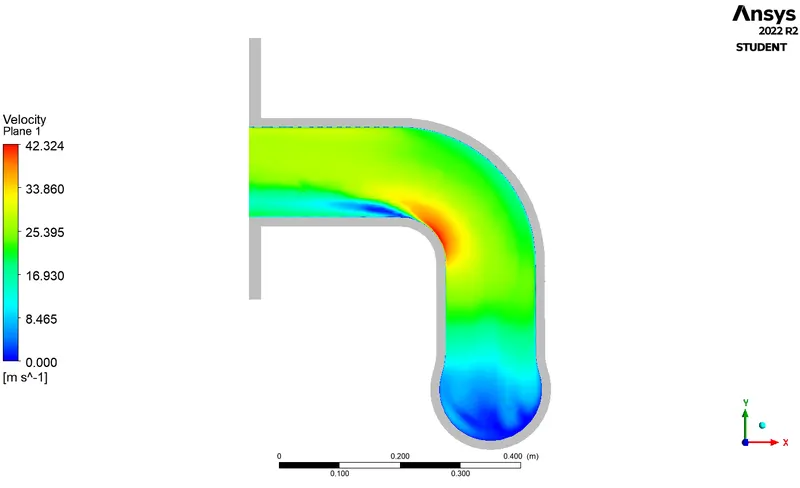
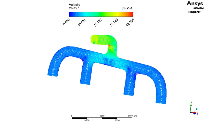
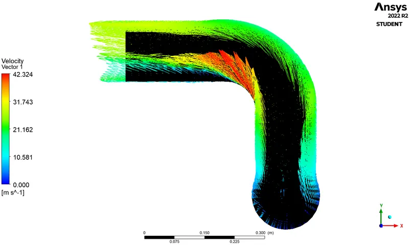
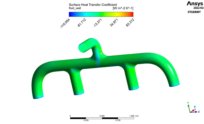
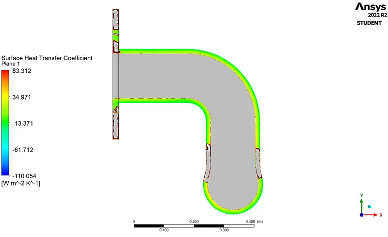
Pressure plots, velocity plots, and temperature plots were observed for the fluid wall and a cut section plane at the outlet. Also, the velocity vectors and the surface heat transfer coefficient were plotted at both locations. To plot the surface heat transfer coefficient, data was imported from the 'Setup' file.


RESULTS -

Contour	Fluid Wall	Outlet (Plane)
Temperature Contour
Pressure Contour
Velocity Contour
Velocity Vector Contour
Surface Heat Transfer coefficient Contour

VALIDATION -

Reynold's number is given as; `Re = frac{rhoVx}{mu}`

`Re = frac{0.7459xx5xx0.16}{2.5677xx10^-5} = 23155.607`

Flow Type	Value of Reynolds Number (Re)
	Laminar Flow	Transitional Flow	Turbulent Flow
Internal Flow	Re < 2300	2300 < Re < 4000	Re > 4000
External Flow	Re < 1 x 105	1 x 105 < Re < 5 x 105	Re > 5 x 105

Thus, the flow is considered as 'Turbulent flow'.

The Dittus–Boelter equation is an explicit function for calculating the Nusselt number.

According to Dittus-Boelter Equation; `Nu = 0.023xxRe^0.8xxPr^n` where `Pr` is Prandtl number for air at `200°C` & n = 0.4 for heating and n = 0.3 for cooling

`=> Nu = 0.023xx23155.607^0.8xx0.6974^0.3 = 64.047`

Also, the heat transfer coefficient for the turbulent flow is `h = frac{kxxNu}{D}` where `k`= thermal conductivity of air at 200°C; `D` = characteristic length of exhaust port pipe

`=> h = frac{0.03779xx64.047}{0.16} = 15.21 frac{W}{m^2 K}`

Value of Heat Transfer Coefficient (W/m²K)
Numerical Solution (`NSol^n`)	Analytical Solution (`ASol^n`)
21.12	15.21

Percentage Difference `= frac{NSol^n-ASol^n}{ASol^n} = frac{21.12-15.21}{15.21} = 0.388 => 39 %`

CONCLUSION -

• According to the conjugate heat analysis phenomenon, the results obtained during the simulation appeared to be relevant.
• Because there is a significant difference between the numerical and analytical solutions, it can be concluded that numerical simulation results for conjugate heat transfer analysis may not be accurate, and only appropriate results can be obtained.
• Thus, one of the inference can be the fact - An analytical solution involves framing the problem in a clear manner and calculating the exact solution. A numerical solution refers to making guesses about the solution and testing whether the problem is well-solved or not.
• Based on the theoretical data and numerical simulation, it is possible to conclude that - The value of the heat transfer coefficients is dependent on the Reynold numbers and Prandtl numbers.

REFERENCES -

• Reference Research Paper
• Fluid Mechanics - Fundamentals and Applications by Yunus A. Cengel & John M. Cimbala
• Heat Transfer - Dr. Thomas Rodger

As a result, Ansys Fluent simulations for Conjugate Heat Transfer (CHT) analysis over an Exhaust Port model was performed, and conclusions were made in consideration of the results.