Week 4 - CHT Analysis on Exhaust port

CHT Analysis on Exhaust port

Aim:To perform CHT analysis on exhaust port using Ansys Fluent.

Objectives:

• To give a brief description of why and where a CHT analysis is used.
• To maintain the y+ value according to the turbulence model and justify the results.
• To calculate the wall/surface heat transfer coefficient on the internal solid surface & show the velocity & temperature contours in appropriate areas.
• To verify if the HTC predictions from the simulations are right and factors associated with the accuracy of the prediction .

Theory:

CHT analysis and its applications:

The Conjugate Heat Transfer (CHT) analysis allows for the simulation of heat transfer between solid and fluid domains by exchanging thermal energy at the interfaces between them. Typical applications of this analysis type exist as, but are not limited to, the simulation of heat exchangers, cooling of electronic equipment, and general-purpose cooling and heating systems.The CHT approach has an advantage over FE thermal analysis in that wall heat transfer coefficients and their local variations on surfaces are directly calculated within the model rather than based on simplified empirical calculations. The CHT approach therefore has benefits for those applications where heat transfer is either non-uniform or difficult to calculate empirically.

Solving and Modelling approach:

Creating Geometry:

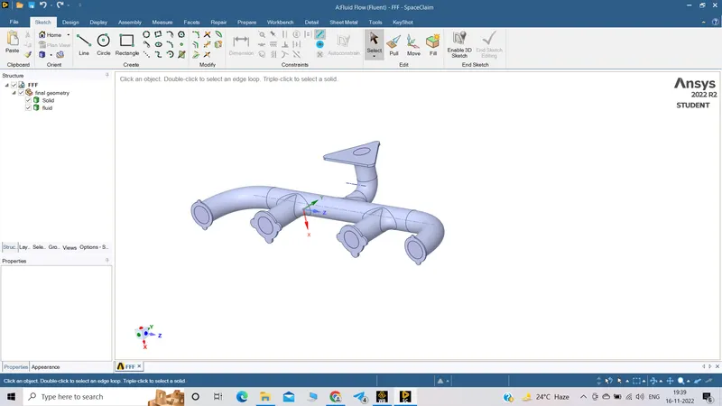
• The exhaust port was modeled into the Spaceclaim by importing the part file.
• The exhaust port is a three-dimensional model containing four inlets and one outlet.
• CHT analysis requires both the solid and the liquid volume under consideration, Spaceclaim gives an option of volume extract for selecting edges for fluid volume.
• Both the solid volume and liquid volume are copied into one component i.e. final geometry.
• Share topology is created.
• Spaceclaim gives an option for share coincident topology, when share coincident topology is selected and executed, the mesh from the fluid volume and the solid volume are said to be conformal with each other which is a requirement for CHT analysis.

Base line meshing :

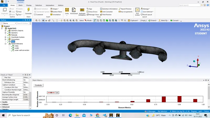
• The exhaust port is loaded into the meshing window and then simulated for baseline mesh and the refined mesh.
• The named selections are created ( inlets, outlet, outer-wall - convection)

Setting up of physics and boundary conditions:

Setting up of physics:

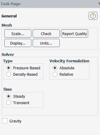
• Energy equation: turned on.

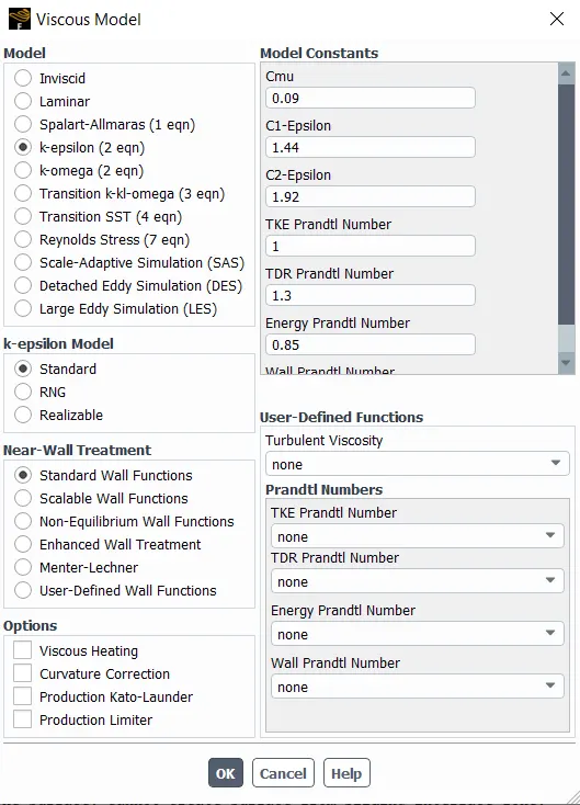
Graphics:

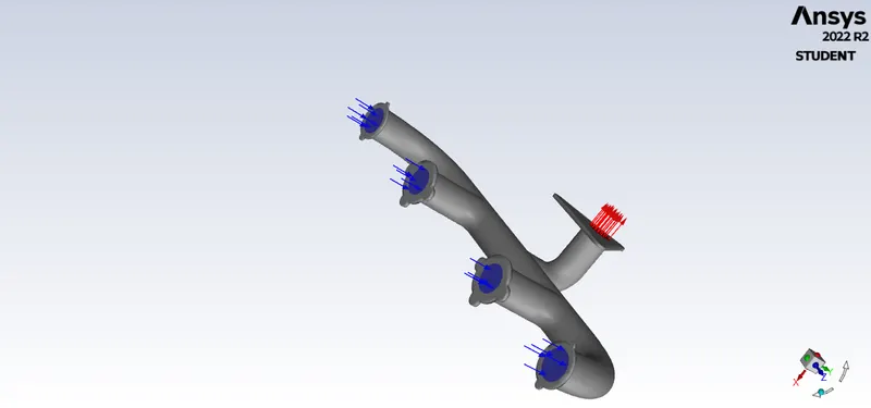
The different boundary conditions are listed below:

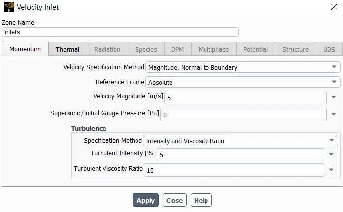
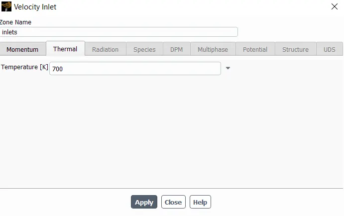
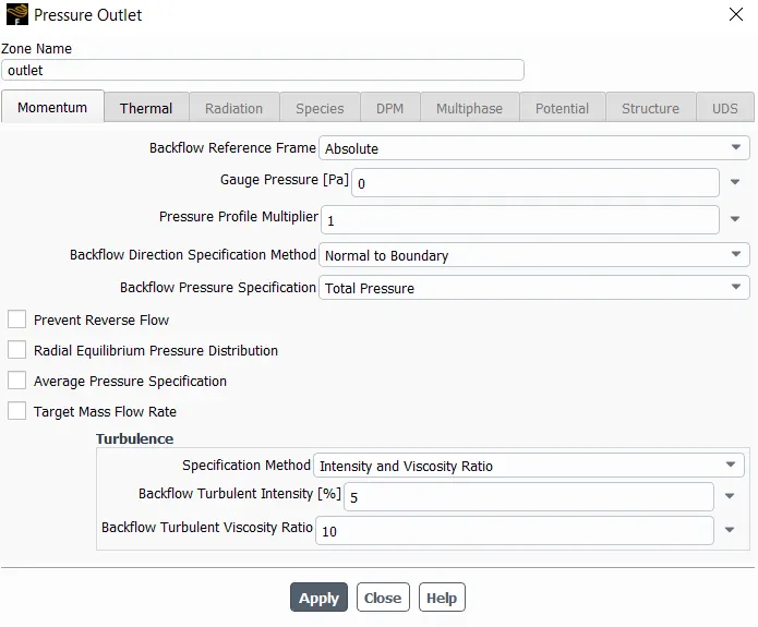
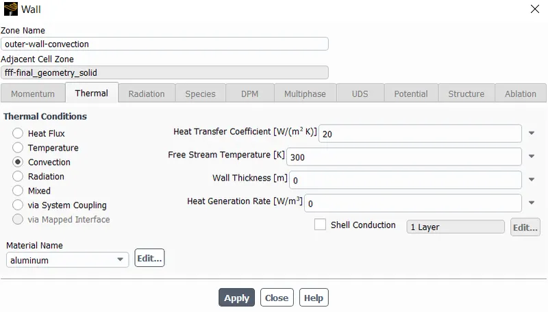
Fluid

• Material Name: Air

Solid

• Material Name: Aluminium

Intialization: hybrid
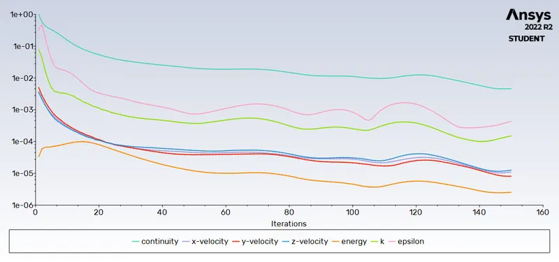
No. of iterations: 150

Solution and Result:

Scaled Residuals:

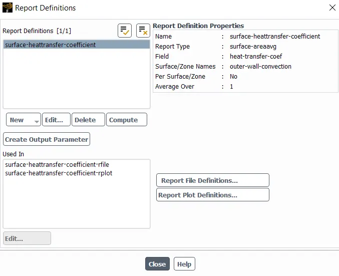
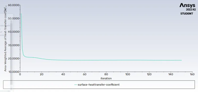
Surface heat transfer coefficient on the internal solid surface :

surface-heattransfer-coefficient 18.663817 W/m²k

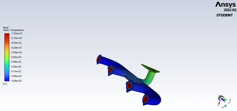
Temperature contour plot:

Surface heat transfer coefficient:

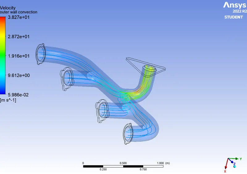
Velocity plot:

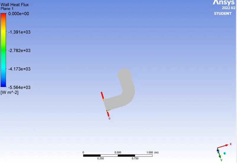
Wall heat flux:

Mesh refinement:

• Inflation layer helps us to create a body fitted mesh.It means it creates a layer of mesh same as the geometry.
• Since at the interface it is very important and we want to calculate the heat transfer at that place we need to take that region and create inflation layers so that flow is captured exactly and the values are calculated exactly.
• To do this we first with selecting fluid part and naming it as inflation layer.
• In the global mesh select inflation option and in that for use automatic inflation - select all faces in the choosen named selection and for named selection - select the inflation layer which we have just named.
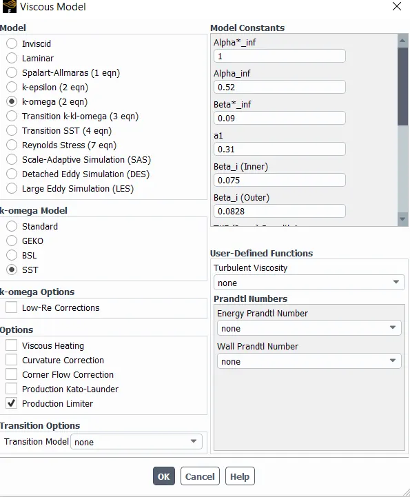
• And for inflation option we use first layer thickness and we give this based on y+ value and the turbulence model we use.Here we use k-omega SST turbulence model so y+ should be in between 0.1 to 5.Lets calculate the first layer thickness.
• U∞ = freestream velocity = 5 m/s
• ρ = freestream density = 1.225 kg/m3
• μ = dynamic viscosity = 0.000017894 kg/m s
• L =diameter of the inlet(m) = 0.1662206 m
• Desired y+ = 1

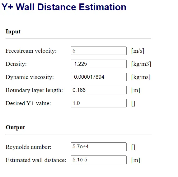
Now we got the first layer thickness 0.051 mm ,let us give the above first layer thickness and maximum of 30 growth layers and with a growth ratio of 1.2 for inflation layers.

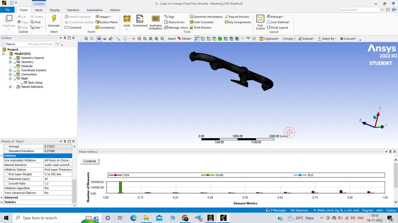
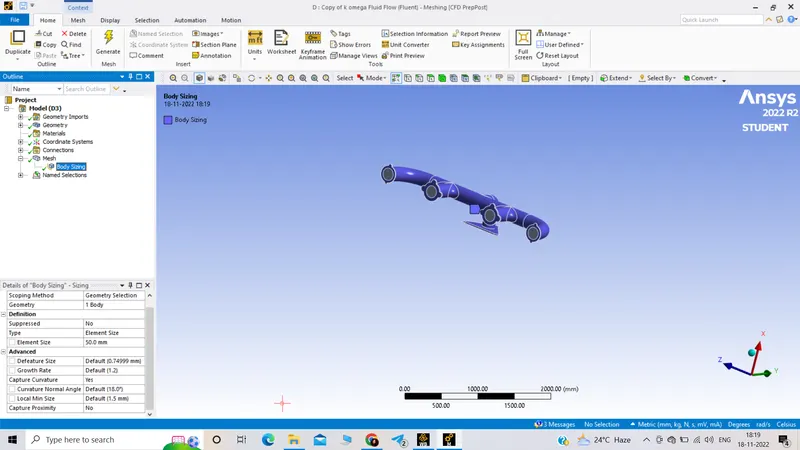
by inserting body meshing element size 50 mm.

Setting up of physics and boundary conditions: k-omega SST

Intialization: hybrid
No. of iterations: 300

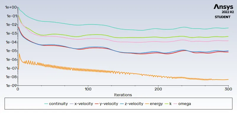
Solution and Result:

Scaled Residuals:

Surface heat transfer coefficient on the internal solid surface :

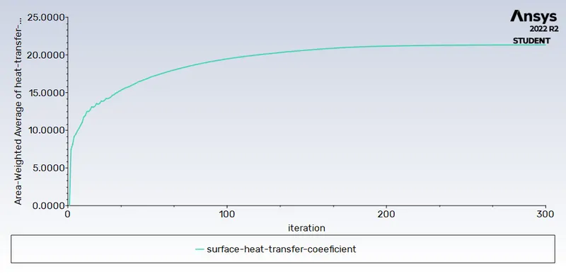
surface-heat-transfer-coeeficient 21.323696 W/m²k

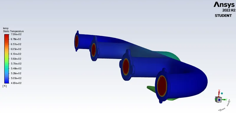
Temperature contour plot:

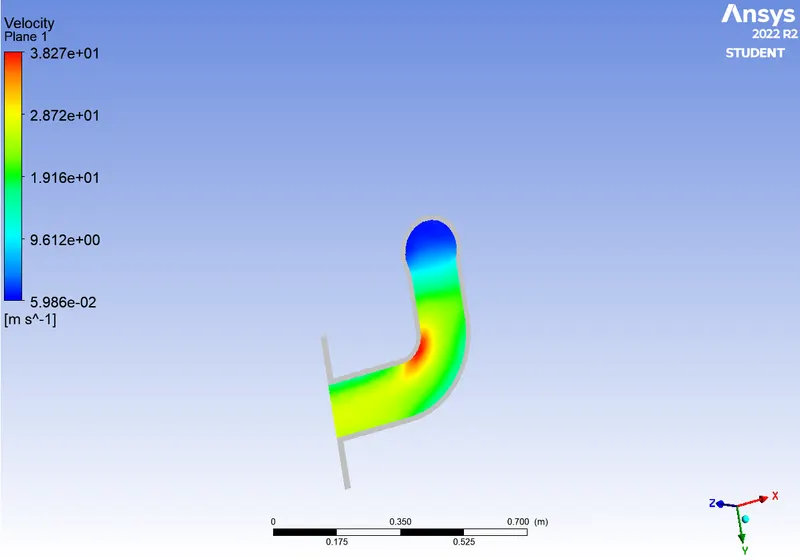
Velocity plot:

Wall heat flux:

Verification of the HTC predictions from the simulations :

According to Bernoulli's mass conservation principle ,

Let us assume the flow rate from each inlet as Q1, Q2, Q3, Q4 respectively, and Q5 be the flow rate from the exhaust manifold.

So,Q1+Q2+Q3+Q4=Q5

`Q=rho AV`

assuming the flow is incompressible,

`A_1V_1+A_2V_2+A_3V_3+A_4V_4=A_5V_5`

At outlet V is high as A is small

`Re=(rhoVD)/mu`

At outlet Re is high as V is high.

As per Dittus Boelter-type correlation,

`Nu=0.023Re^0.8Pr^n=(hD)/k`

Where Nu = Nusselt number; Re = Reynolds no.; Pr = Prandtl number; h = heat transfer coefficient(W/m²k); and D = inner diameter of the tube (m).n=heating exponent k= constant thermal conductivity

`Nuprop Re;Re prop h`

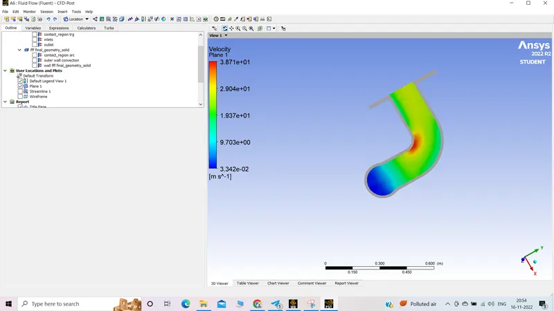
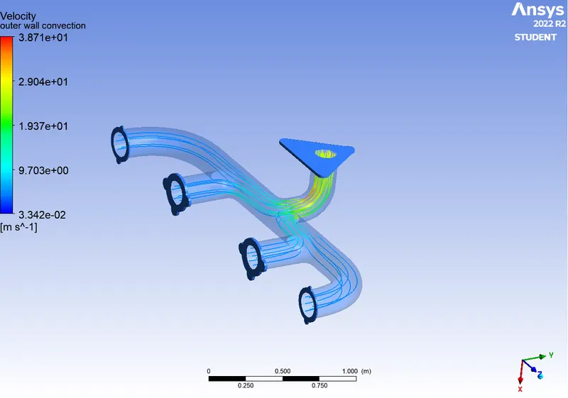
From our simulation, we have observed velocities are high at bend section of outlet manifold hence higher Reynolds number so heat transfer coefficient is also high.

Nu=`0.023*57000^(.8)*0.744^(0.3)=134.24`

pr=`(mu*cp)/k`

mu=`1.789*10^-5`

cp=1006.43 J/kg-k

k=thermal conductivity = 0.0242 w/mk

pr=`(1.789*10^-5 *1006.43)/0.0242=0.744`

Nu=`(hD)/k`

h=`(134.24*0.0242)/0.166=19.57`W/m²k

Analytical h=19.57 W/m²k

Simulated h= 18.663817W/m²k(base line meshing)

Simulated h= 21.323696 W/m²k(refined meshing)

Nearly same(Result is correct)

The Dittus-Boelter correlation may be used for small to moderate temperature differences, T_wall – T_avg, with all properties evaluated at an averaged temperature T_avg.

For flows characterized by large property variations, the corrections (e.g. a viscosity correction factor μ/μ_wall) must be taken into account, for example, as Sieder and Tate recommend.

When the difference between the surface and the fluid temperatures is large, it may be necessary to account for the variation of viscosity with temperature. Therefore a modified form of Dittus-Boelter equation was proposed by Sieder and Tate (1936).

Sieder-Tate equation:

`Nu=0.027*Re^(4/5)*Pr(1/3)*(mu/mu_s)^0.14`

Validity:

0.7≤Pr≤16700

Re>10000

L/D> 10