Week 4 - CHT Analysis on Exhaust port

Aim/Objectives

To understand why and where a CHT analysis is used.

To calculate the surface heat transfer coefficient on the internal surface of the given exhaust port.

Verify the HTC predictions from the simulations and validates its accuracy.

Introduction

CHT analysis

The word CHT stands for Conjugate heat transfer.

Conjugate Heat Transfer is a analysis of heat transfer between a solid and fluid domain by exchanging the thermal energy at the interface between them.

Typical application for this analysis type are simulation of heat exchangers, cooling of electronic equipment and general-purpose cooling and heating systems.

Solving and modelling approach

The work flow for CHT analysis on a exhaust port

• Pre-processing
• Solving
• Post processing

Pre-processing and solver setting

Initially in pre-processing the geometry of the exhaust port is imported into ansys workbench.

Geometry

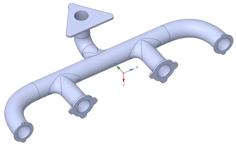
With the help of spaceclaim geometry is edited.

Here the fluid volume is extracted with the help of volume extract tool.

Fluid volume

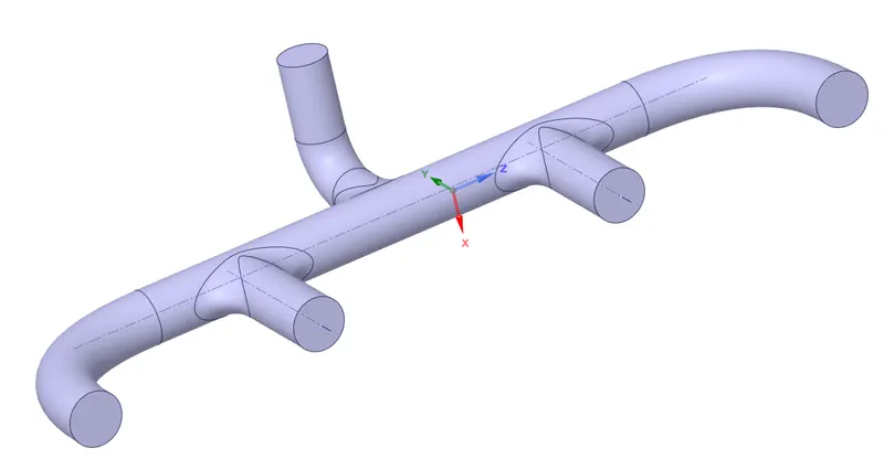
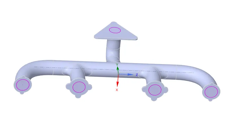
After extracting the fluid volume share topology is enabled to share its topology with its neighbouring faces.

The pink colour in the geometry indicates that it has shared its topology.

Mesh

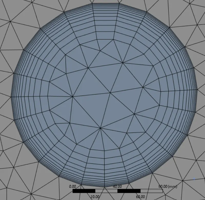
Mesh is generated with tetrahedral elements.

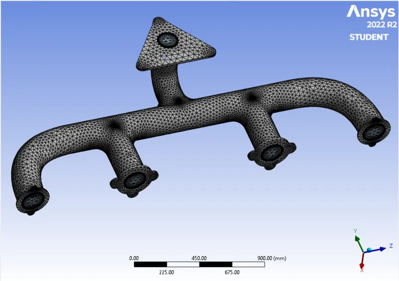
Inflation layer are generated in order to capture the properties at boundary clearly.

For this in inflation option first layer thickness with first layer height of 0.6 mm and maximum layers of 12 with growth rate 1.25 is choosen.

The solver type used here is pressure based and steady state solver.

Energy equation is turned on as temperature is involved and K omega SST Tubbulance model is used.

Material(Fluid) is air. Its inlet velocity is about 5 m/s and temperature of 700 k.

Other boundary conditions like outer wall convection in which wall convection is set to 20 W/m²K.

Numerical approach

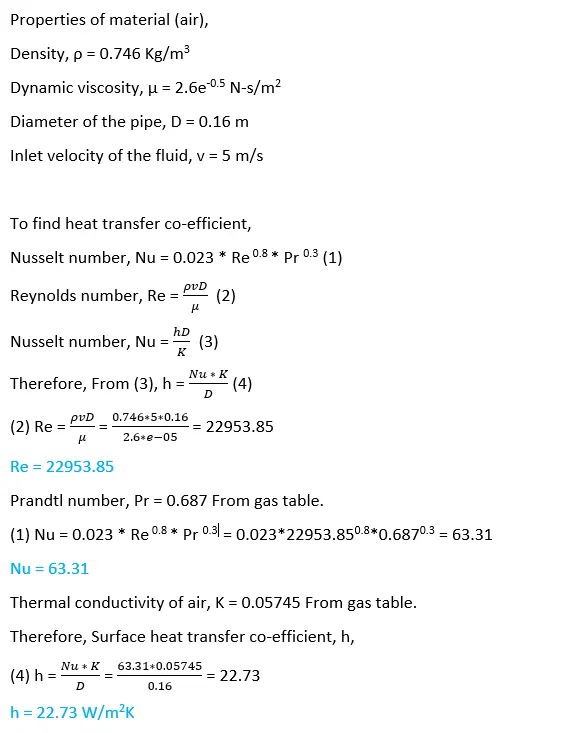
In order to verify the HTC predictions from the simulations and validates its accuracy numerical approah is used.

Results

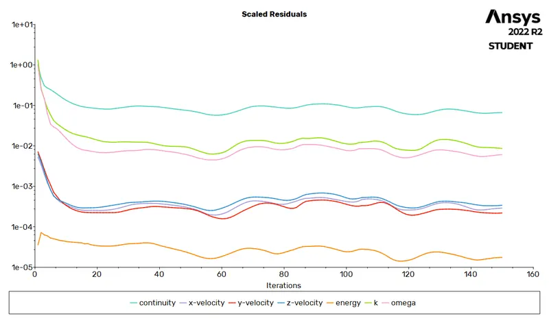
Residuals

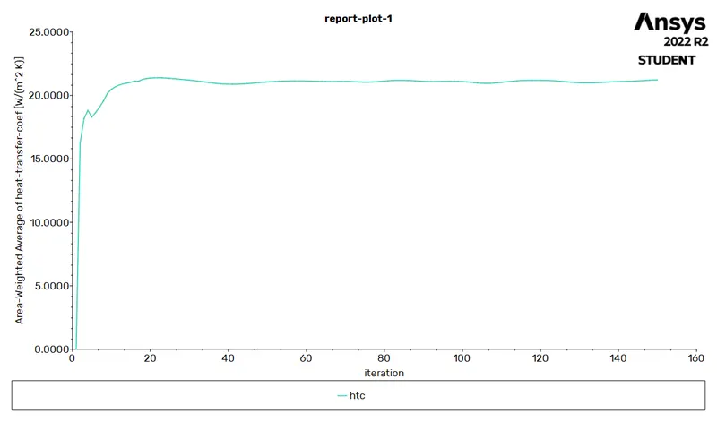
Area weighted average of heat transfer coefficient

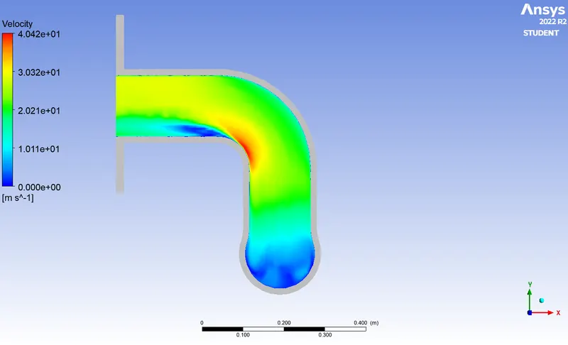
Velocity contour

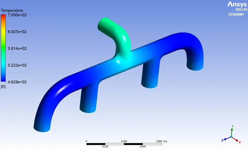
Temperature contour

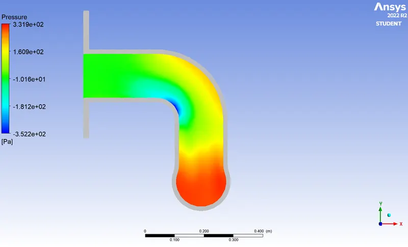
Pressure contour

Surface heat transfer coefficient

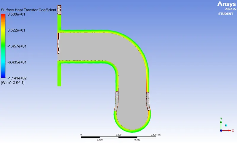
Surface heat transfer coefficient is maximum near to the walls because of that is were the velocity is maximum.

Conclusion

Surface heat transfer coefficient for numerical approach is about 22.73 w/m²k.

Surface heat transfer coefficient for simulation approach 21.22 w/m²k.

From the above table surface heat transfer coefficient of numerical results matches well with the simulation results with an error of about 1.51.