Week 4 - CHT Analysis on Exhaust port

Aim- To perform a steady state conjugate heat transfer simulation on the exhaust port when the air is coming at a speed of 5m/s.

Objective-

1. Explain Conjugate Heat transfer analysis

2. Solving and modelling approach.

3. Simulate the wall/surface heat transfer coefficient on the internal solid surface

Explanation-

1. Conjugate Heat Transfer Analysis- It is based on the mathematical structure problem which describes the heat transfer between the body and the fluid flowing over or inside it as a result of the interaction of two objects of the matching interface eliminating the need to calculate the heat transfer coefficient.

Conjugate Heat Transfer Analysis allows for the simulation of the heat transfer between the solid and the liquid domains by exchanging thermal energy at the interface between them.

In the case of CHT here the project has been done by the convection mode of heat transfer between fluid and the solid Aluminium wall of the exhaust pipe then the convection mode is followed within the wall of the exhaust pipe.

Solving and Modelling Approach-

The exhaust pipe has been imported on the space claim.

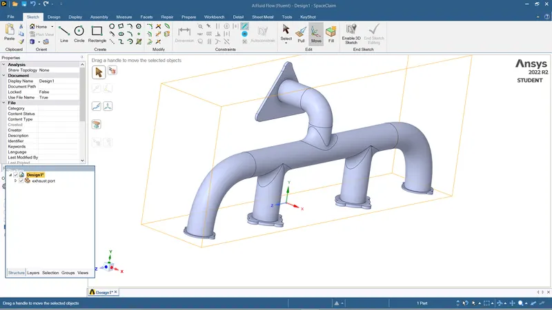
The exhaust pipe is a 3d model consisting of four inlets and one exhaust as an outlet. despite having an isothermal boundary condition and a uniform flow rate at the four-inlet model can not be cut into halves to reduce the computational power. Therefore the exhaust pipe has to be discretised as it is thus this is called space discretization.

By using the volume extract option on the space claim extract the fluid geometry form the solid geometry. because we need a fluid and solid geometry defined for the CHT to study the flow and temperature difference according to the geometry.

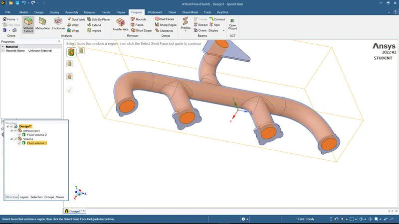
We combine the both fluid and solid components a named it under one new component i.e; Final geometry.

And make sure the shared topology is enabled so that while meshing the meshed triangle should not be intersecting each other boundaries.

Meshing-

Import the modified geometry in the mesh for meshing the geometry.

At first named all the entities as- inlet, outlet, outer convection wall

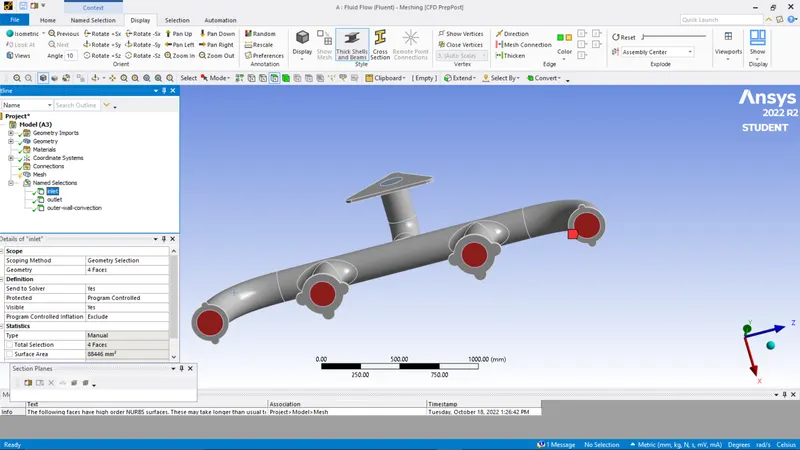
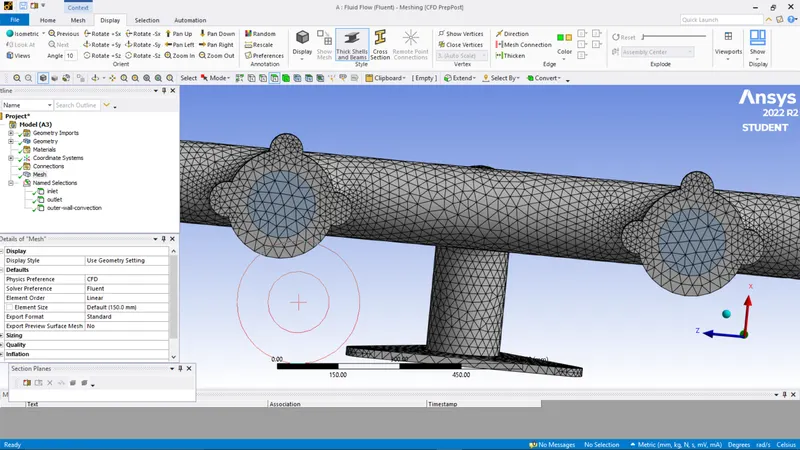
Then generate the mesh and check if the mesh performed is correct or not. And also make sure the mesh generated is Conformal Mesh(that the meshing entities is purely defined and no intersections in meshing trias)

Setup-

Import the meshed geometry into the Ansys fluent.

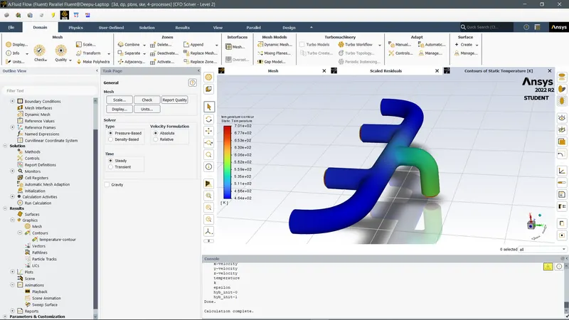
Perform the simulation with the viscous model as K-epsilon, steady state analysis and with a Pressure based Solver. and make sure the solution is been select Simple Solution.

Boundary conditions-

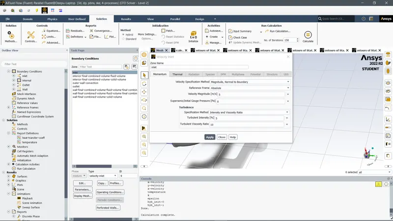
inlet---Velocity-5 m/s,Thermal- 700k

Outlet---pressure- 0 pascal

Outer wall Convection---edit- convection- heat transfer coefficient= 20

Final Boundary-- heat flux

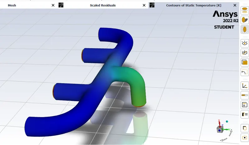
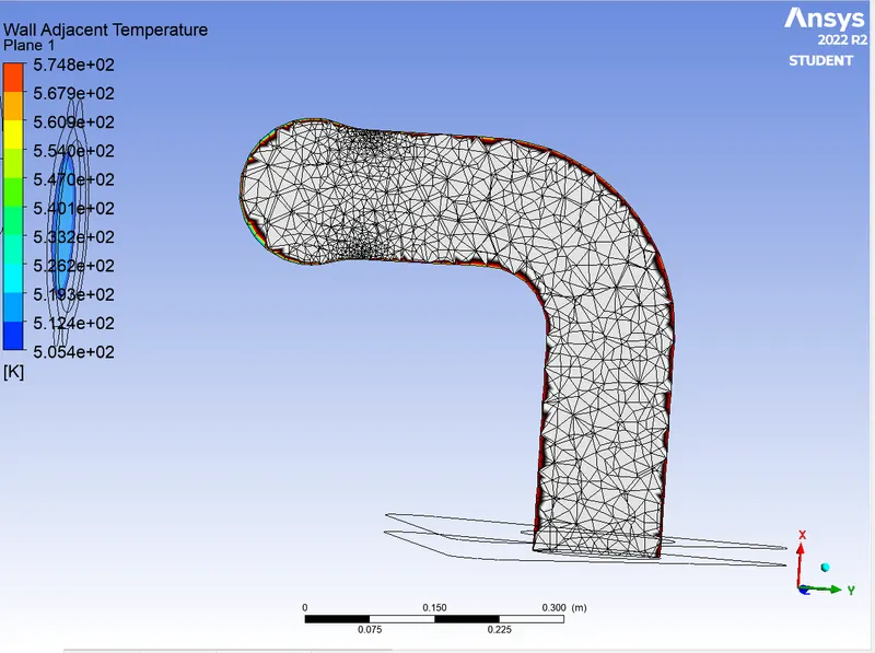
As we can see that the temperature difference from the convective heat transfer is not been clearly captured because of the less cell counts on the meshed geometry because of this meshed geometry is not able to capture all the deatails.

Case-2

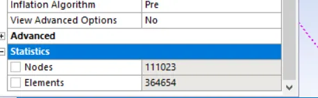
We make an inflation layer in the fluid geometry so the edges will be more defined while running the simulation and also try to reduce the mesh sizing of the outer geometry so that we can capture more details on the Conjugate Heat transfer analysis.

The inflation layer is added to the fluid geometry by = 6 layers, Growth rate = 1.2 and First layer thickness=0.05mm

capture curvature= Yes(so that the mesh generated will try to capture all the curavtures.)

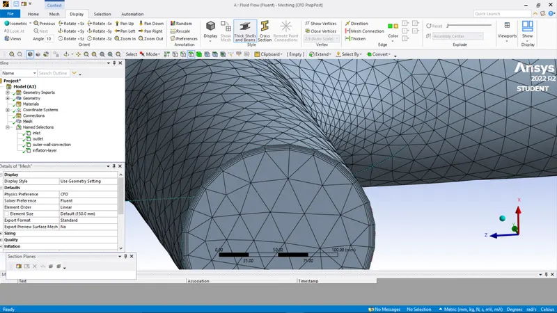
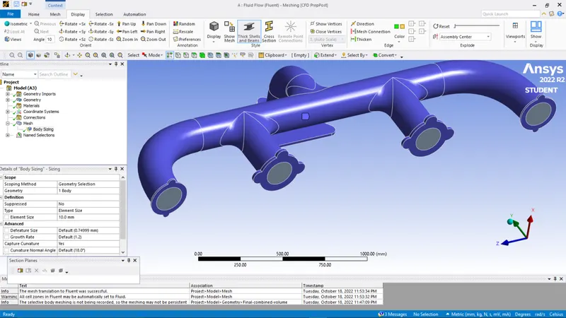
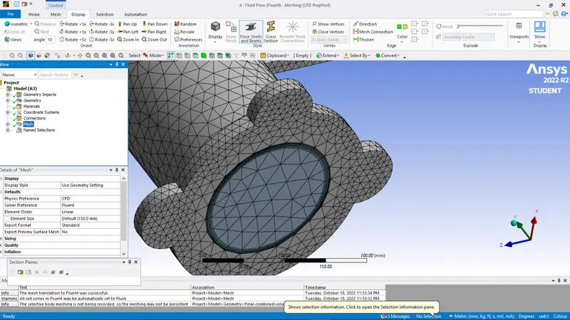
Mesh is being generated.

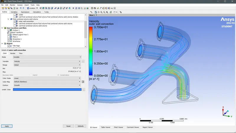
We run the setup again with the same solver and same boundary conditions, the results obtained as-

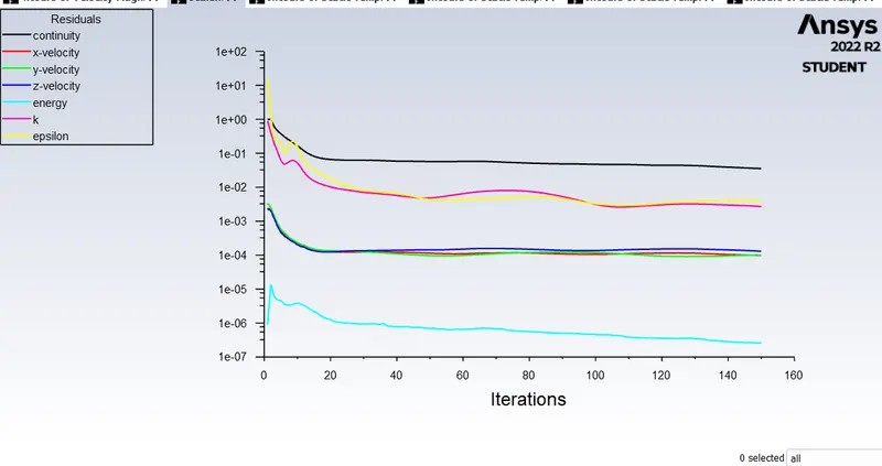
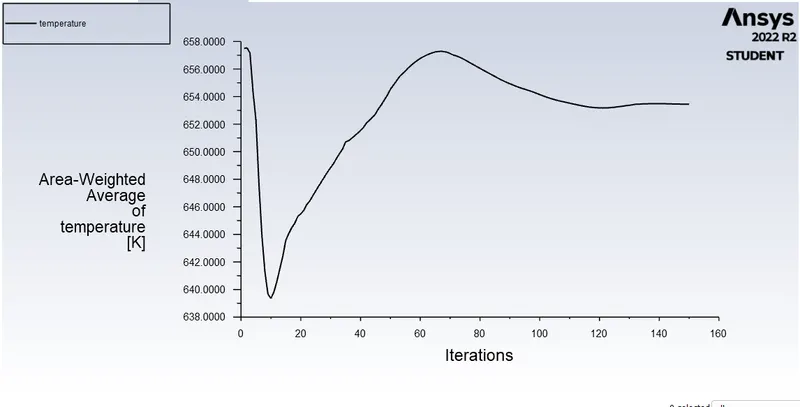
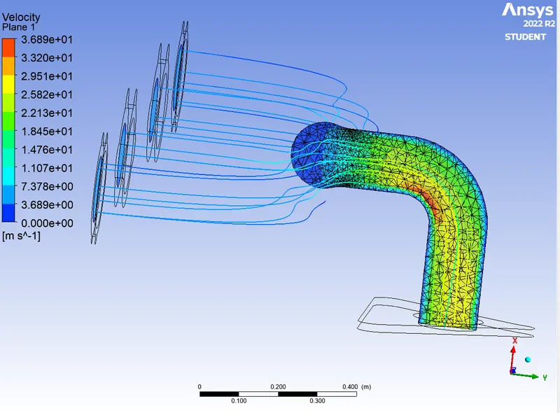
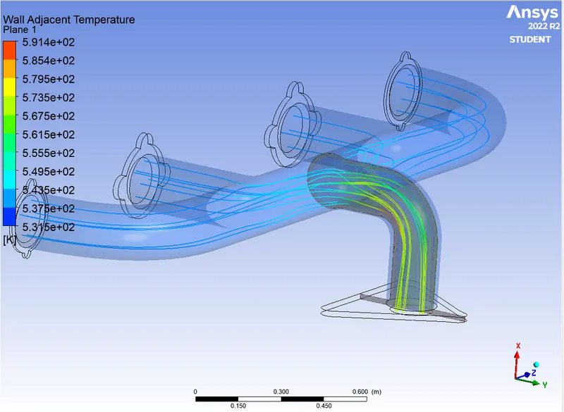
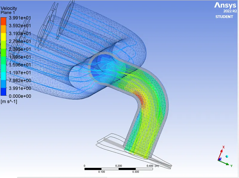
With this contour plot, the point of the localized heat flux source is maximum at the turning point which denotes that the same point of maximum velocity will be the point of maximum heat transfer.

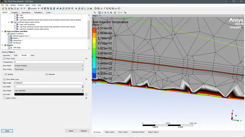
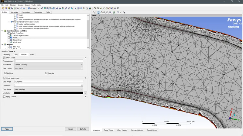
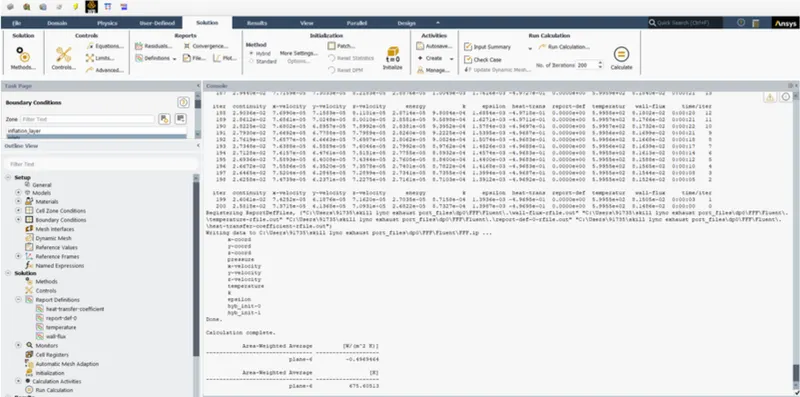
The area weighted average heat transfer coefficient= 0.469w/m^2k and Area weighted average of the temperature= 475.40k

In the analysis,the heat transfer coefficient is of h=20.66w/m^2-k

Analytical Solution-

Reynolds number of the flow is of Re=56867.66 at flow velocity = 5m/s.

By using Dittus Bolter heat transfer coefficient relation in natural turbulent flow the ditus bolter HT coefficient is determined by the nusselt number which is related by the formula of

Nu(D)= 0.023*Re^(4/5)*pr^n here n= 0.3, Dia(diamter of the pipe=characteristic length) = 0.166m

The prandtl Number is

pr=mu*cp/k here mu=1.789*10^-5 Cp=1006.43 J/kg-k and k= thermal conductivity =0.0242w/mk

pr = (1.789*10^5*20)/0.0242= 0.744

The nusselt number is calculated as

Nu = hD/k = 131.792 = h*0.166/0.0242 = 19.52 w/m^2k

Conclusions-

• the theoretical value and the computational value of the thermal specific heat transfer coefficient to be = 19.52 so the computational way which is 20w/m^2k is closed.
• By using the finer grid and inflation layer by reducing the element size we abled to capture more accurate details with much less deviation.
• The value of heat transfer coefficient of the wall allows us to choose the value of y+ =1 for the turbulence model.
• The presence of the boundary layer is quite visible near the inlet of the wall because the velocity is near to zero. and near the outlet the velocity is highest. so giving the highest reynolds number.