Week 4 - CHT Analysis on Exhaust port

The aim of this exercise is to conduct a conjugate heat transfer analysis (CHT) on exhaust port.

CHT analysis is used to obtain high resolution thermal inputs on wet surfaces since standard process uses constant heat transfer coefficients and not the nodal heat transfer coefficients.In cht analysis, we can solve both the solid and fluid flow areas simultaneously and obtain accurate heat transfer results. Some of the examples are forced convection used in fins, conduction between two solids, and gases.

For this simulation, a model of an exhaust port is made and imported into ansys spaceclaim. Now, after importing the model, we can extract the fluid volume by using volume extract options under prepare. After extracting the fluid volume, the geometry is checked for duplicates and then the solid volume as well as the fluid volumes are moved under a single topology and the share topology option is enabled. Then, we enable shareprep and share the topology between the solid and fluid volumes and save the file to proceed further to meshing.

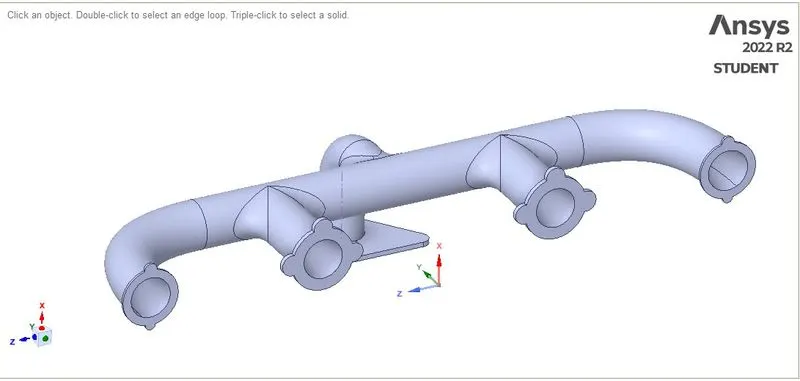
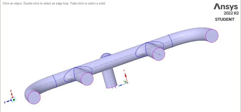
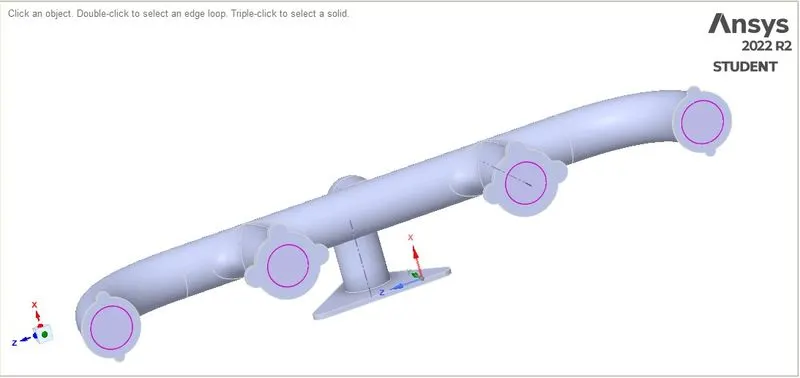
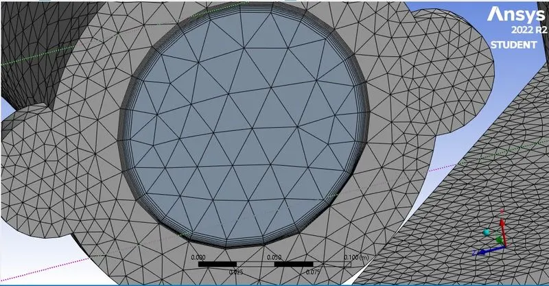
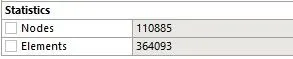
Once the model has been imported into meshing, we can create named selections for the inlets, outlets, outer walls, and inflation layers. Then, we provide the sizing for the mesh and insert a method for sizing, and by selecting the whole body, we provide a mesh size of 10mm. We also add inflation layers with growth rate =1.2 and 5 layers. Now, we generate the mesh and then move to fluent.

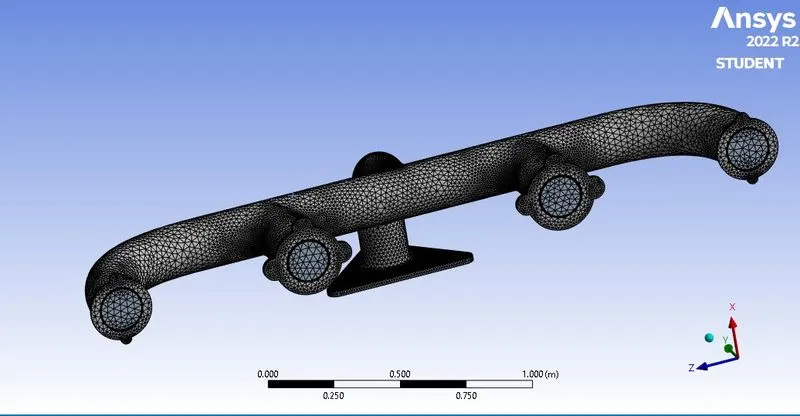
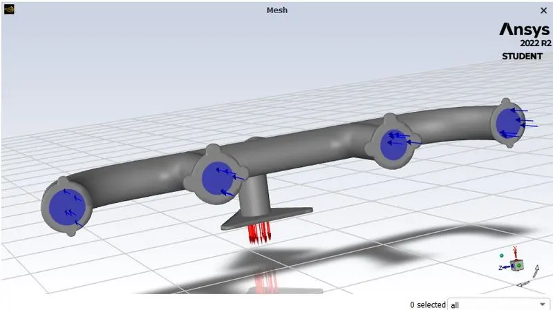
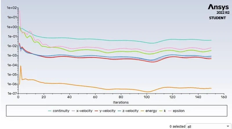
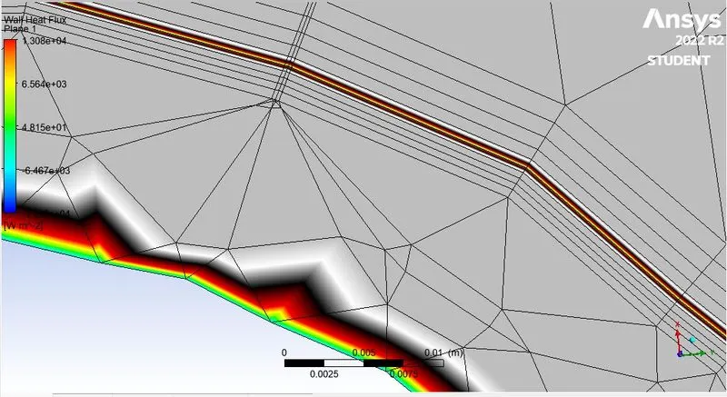
Now, in fluent, we provide all the necessary boundary conditions and specify all the parameters that are required to conduct the simulation. we first provide the materials for fluid and solid as air and aluminium. Then, we choose steady state,pressure based absolute velocity formation solver with k-epsilon turbulence viscous model as solver and energy equation enabled. Then, we Move to cell zones and boundaries where we seet the inlet velocity boundary condition as 5m/s and temperature of the incoming fluid as 700K. Then, for outer wall convection, we set the heat flux as 10 kgs^3 and then initialize the solution with hybrid initializtion. Now, we can set the temperature and heat transfer coefficient plots that are required and set an animation for the plots and run the solution for 150 Iterations.

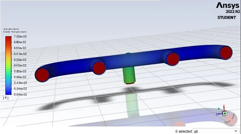
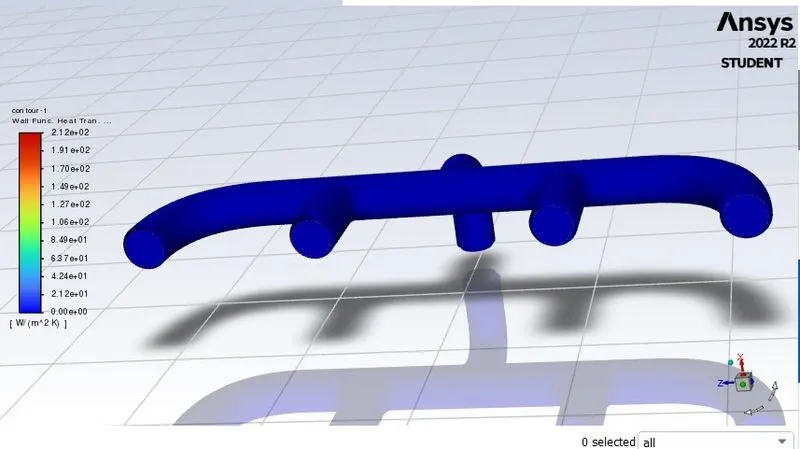
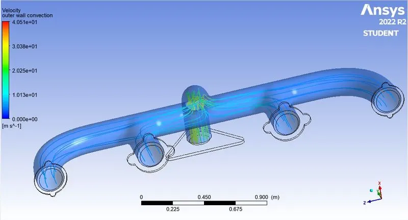
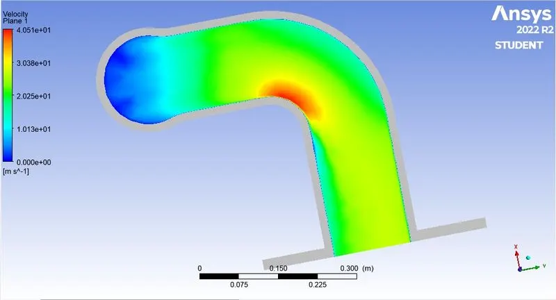
We can calculate the analytical solution for heat transfer coefficient as follows:

Prandtl no Pr = `mu`*cp/k where `mu`= 1.78*10^-5; cp = 1006.43 J/kgK; K = 0.02 W/mK

therefore Pr = 0.74;

Now, Nusselt no. Nu = 0.023*Re^(4/5)*(Pr^n) where D is the dia of the piper and n =0.3;

Therefore, Nu = 131.7 and now, Nu = (h*D)/K where h = heat transfer coefficient,

Therefore, from the above equation, h = 19.5W/m^2K.

From the simulation, the value for heat transfer coefficient is obtained as 21.2 W/m^2K.

Now, comparing both the results, we can find out the error and finally calculate the actual difference between the simualtion and analytical data for discrepancy. Also, the accuracy of the results depend upon the y+ factor. Without the inflation layers, the results obtained are quite vague and when the inlfation layers are added while the mesh size is refined, we can control the accuracy of the solution obtained and the discrepancy between the simulation and analytical results tend to decrease by doing so. In this case, the deviation between the solution is less and hence provides us quality results.