Week 4 - CHT Analysis on Exhaust port
What is CHT Analysis, Why and Where it is used?
Conjugate Heat Transfer (CHT) refers to the coupling of conduction in solids with the convective and radiative heat transfer in the surrounding fluids. In other words, CHT corresponds with the combination of heat transfer in solids and heat transfer in fluids. In solids, conduction often dominates whereas in fluids, convection usually dominates. Efficiently combining heat transfer in fluids and solids is the key to designing effective heaters, coolers, or heat exchangers. Heat transfer in solids and heat transfer in fluids are combined in majority of applications. This is because fluids flow around the solids, or between solid walls, and because solids are usually immersed in a fluid.
The CHT Analysis is used in processes which involve variations of temperature within solids and fluids, due to thermal interaction between the solids and fluids. The exchange of thermal energy between the two physical bodies is called study of Heat Transfer, the rate of transferred heat is directly proportional to the temperature difference between the bodies. A typical example is the heating or cooling of a solid object by the flow of air in which it is immersed.
The physics of conjugate heat transfer is common in many engineering applications, including heat exchangers, HVAC, and electronic component design.
Here we are conducting an analysis on the exhaust port of an engine. The Geometry of the exhaust port is in the image below. With this analysis
we can find out the Heat transfer coefficient.
The heat transfer coefficient or film coefficient, or film effectiveness, in thermodynamics and in mechanics is the proportionality constant between the heat flux and the thermodynamic driving force for the flow of heat (i.e., the temperature difference, ΔT):
The overall heat transfer rate for combined modes is usually expressed in terms of an overall conductance or heat transfer coefficient, U. In that case, the heat transfer rate is:

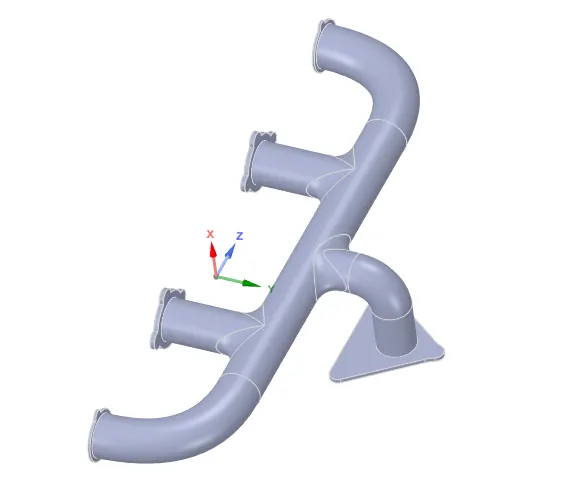
As you can see this exhaust port has 4 inlets and one outlet which then goes to the down pipe and then a catalytic converter,Which is followed by the end can.
So, What we are simulating is that hot air of 700K (approx. 420degree celcius) at a velocity of 5m/s. Then we get the value for the heat transfer coefficient.
We Use K-Epsilon model with scalable wall functions (default option in new version of Fluent). It will keep the Y+ above 11.06 so that it does not suffer the limitation of old standard wall functions.
hybrid wall function is applicable for all Y+ values. But keep in mind that these hybrid wall functions are designed for SA and K-Omega type models (SST included). However, K-Epsilon type models are designed for wall functions i.e. Y+ >30. But with one equation treatment for K-Epsilon models you can integrate them to viscous sub-layer. In this case K-Epsilon type models requires Y+<0.2. This is also known as enhanced wall treatment.
you can see that, strict value of Y+ < 2 for SST model and Y+ < 1 for SA model is now not must. So keeping Y+ upto 10 will give you same results as of mesh with Y+ ~ 1. Also note that for transition modeling (laminar to turbulence transition) you need mesh with Y+ < 1 everywhere along with the requirement of fine mesh in stream-wise direction.
Case 1
baseline mesh and no inflation layer.
Geometry
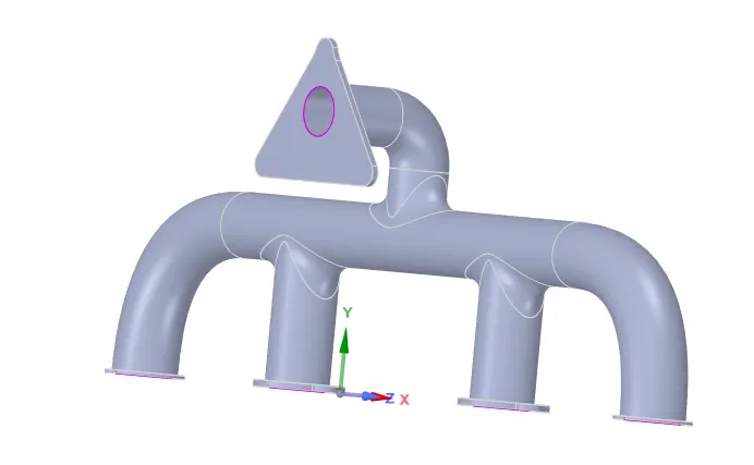
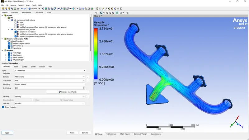
The above geometry represents an exhaust port with 4 inlets and 1 outlet. which are shown below. The idea is so simulate the flow of hot gasses(in this case air) and see how the temperature and the velocity vary. It is made of aluminium and passes hot air in this simulation.
BC For inflation layer
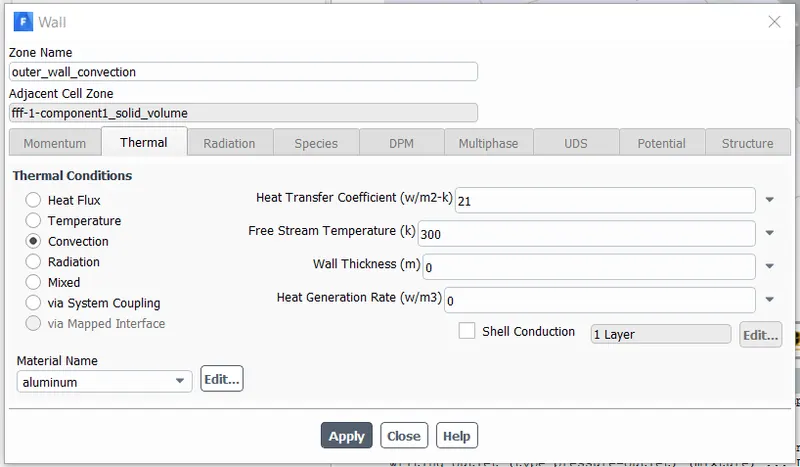
Heat transfer coefficient taken as 21.
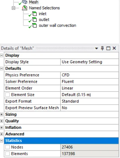
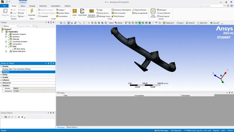
Mesh (Baseline automatically generated)
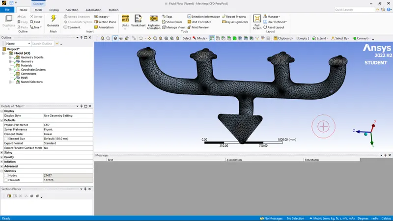
Inlet boundary condition (velocity inlet) @ 5m/sec
Outlet (Pressure outlet) Gauge pressure 0Pa
Outer wall convection (Heat transfer coefficient 20(Wm2k)20(Wm2k) free stream temperature 300K)
The flanges around the inlet and the component encompassing the outlet are adiabatic (no heat transfer takes place through these walls).
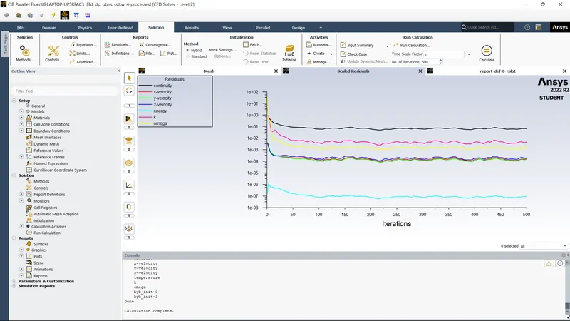
Residual plot
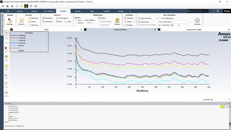
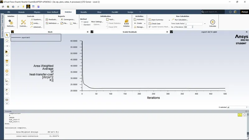
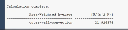
Heat Transfer coefficient
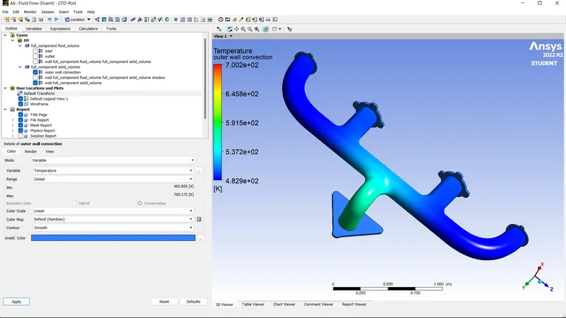
Temperature
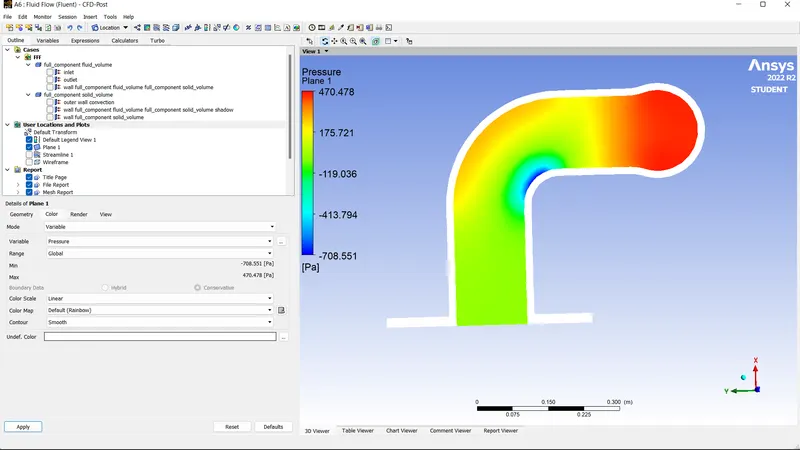
Pressure Plane
Velocity
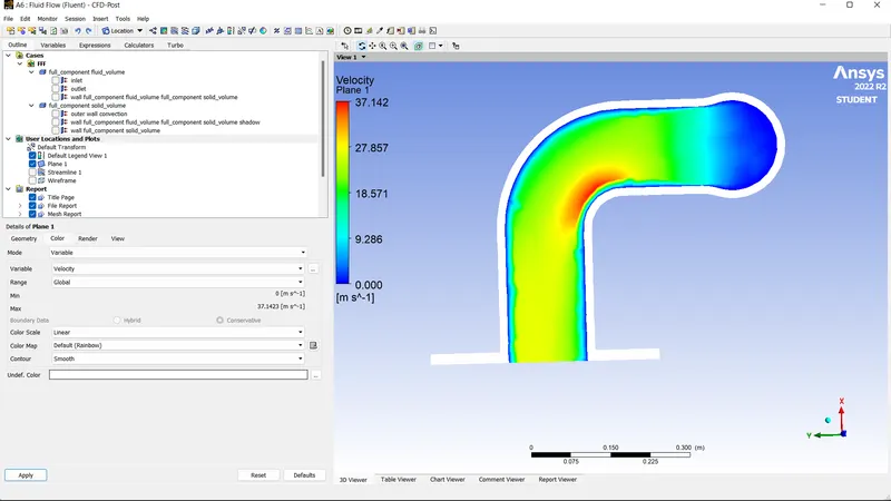
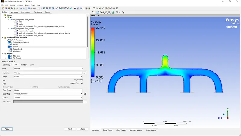
Wall Heat transfer
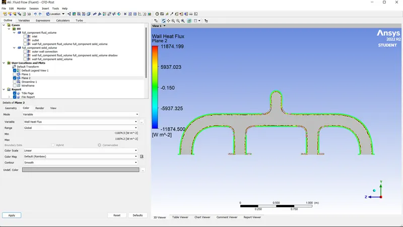
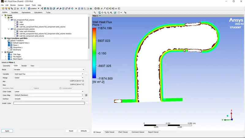
Heat Transfer coefficient
|
Heat transfer coefficient |
21.926374 (Wm2k)(Wm2k) |
CASE 2
A.First refinement
Element size: 90mm
Since the value of the heat transfer coefficient takes the value of the first cell near the wall, so it can be inferred that the Y+ value will be in the viscous sub-layer which is taken to be 1.
Steps involved in calculating the first cell height.
Reynolds number= ρ∗v∗Lμρ∗v∗Lμ
=1.225∗5∗0.171.7894e−051.225∗5∗0.171.7894e-05
=58189.896058189.8960
The characteristics length is taken as the inlet dia.
Skin friction coefficient, Cf=0.058R0.2eCf=0.058Re0.2
=0.00646=0.00646
Wall shear stress formula, τw=0.5∗Cf∗ρ∗v2τw=0.5∗Cf∗ρ∗v2
=0.5∗1.225∗25∗0.006460.5∗1.225∗25∗0.00646
=0.0989Pa0.0989Pa
Frictional velocity formula, uτ=(τwρ)0.5uτ=(τwρ)0.5
=0.2841msec0.2841msec
Now,Y+=△y∗uτ∗ρμY+=△y∗uτ∗ρμ
Since Y+=1Y+=1
Therefore △y=μuτ∗ρ△y=μuτ∗ρ
=0.0000514162m0.0000514162m
=0.05141621mm0.05141621mm
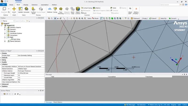
Inflation
Number of inflation layer: 6
Growth rate: 1.2
Inflation option: First layer thickness
First layer thickness: =0.05141621mm
Captured curvature is set to yes.
Body Mesh
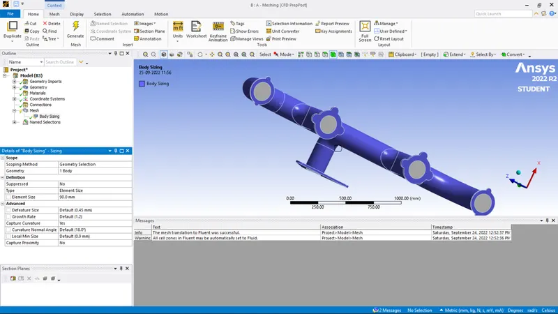
Inflation layers
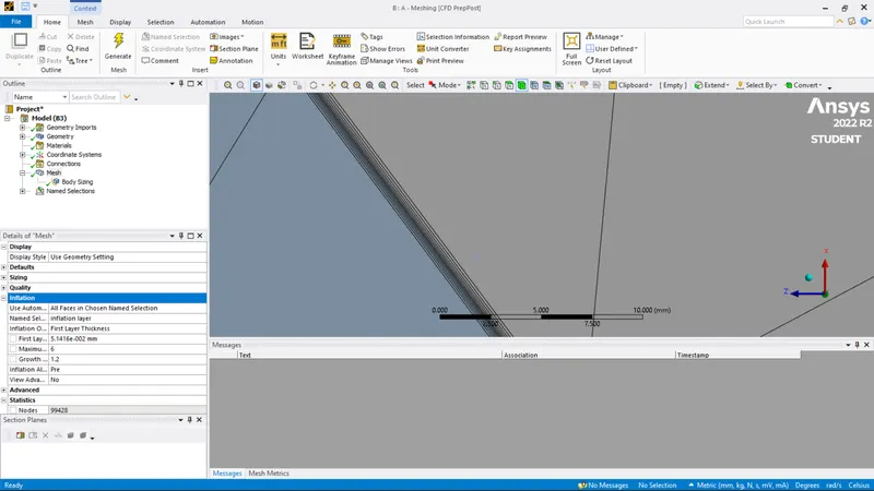
Mash
Residual plot
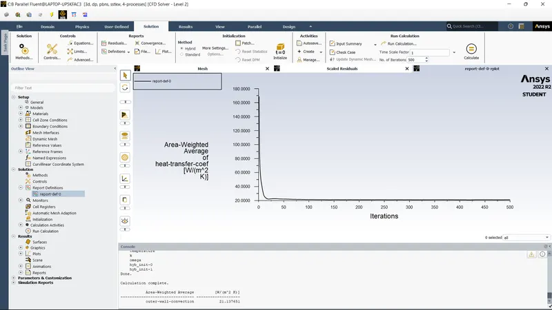
Heat Transfer coefficient
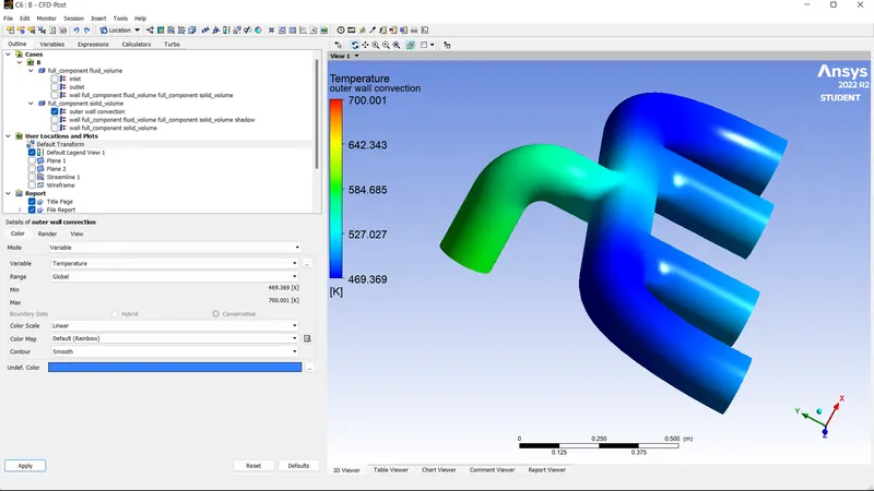
Temperature outer wall convection
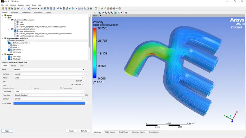
velocity
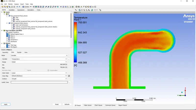
Temperature plane
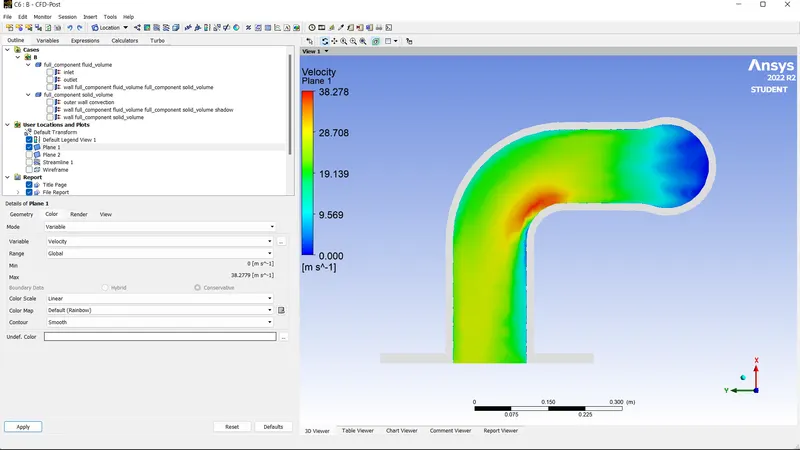
Velocity
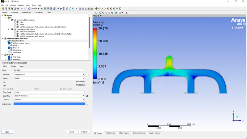
Heat transfer
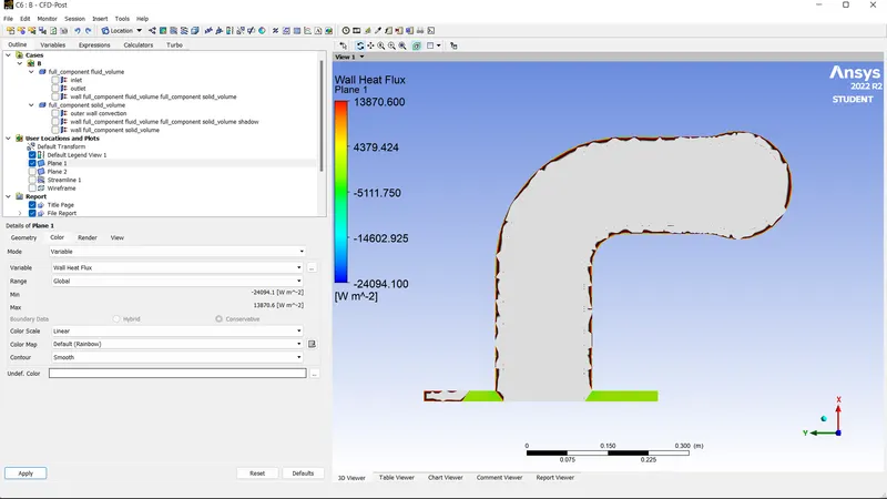
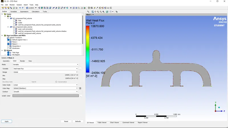
Heat Transfer coefficient
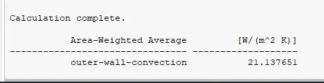
|
Heat transfer coefficient |
21.137651 |
B.Second refinement
Element size: 80mm
Number of inflation layer: 10
First layer thickness:0.05141621mm
Growth rate: 1.2
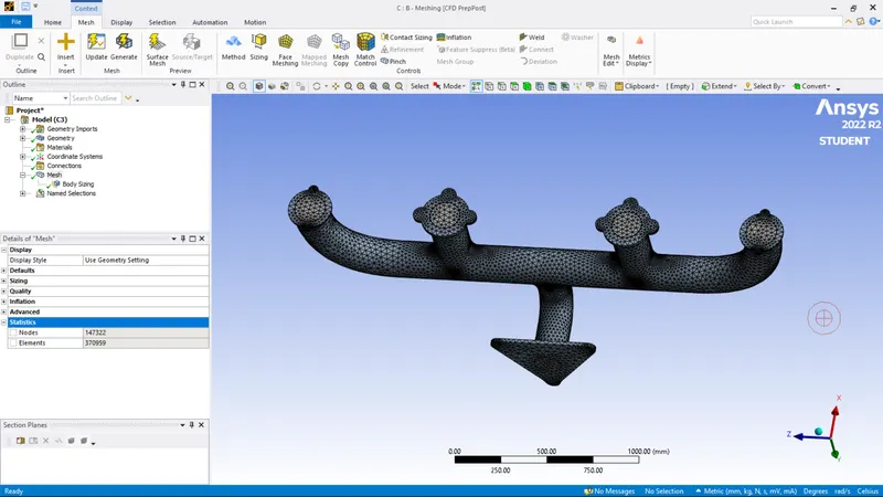
Inflation layers
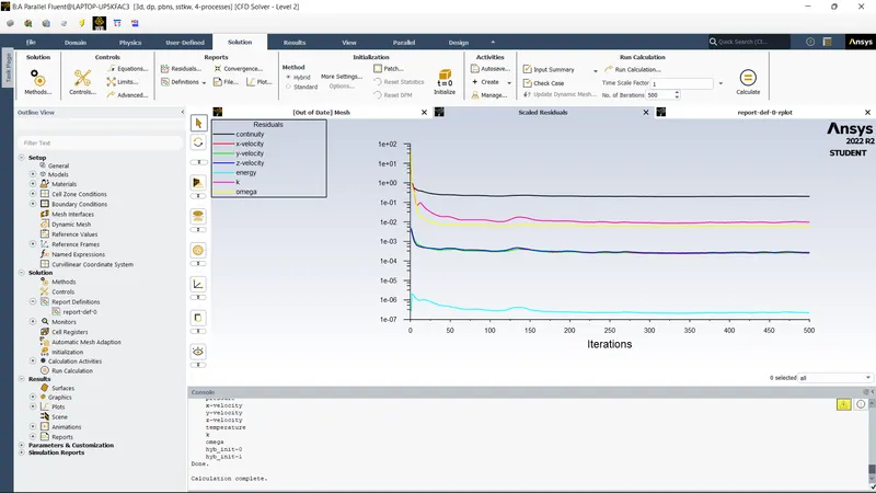
Residual plot
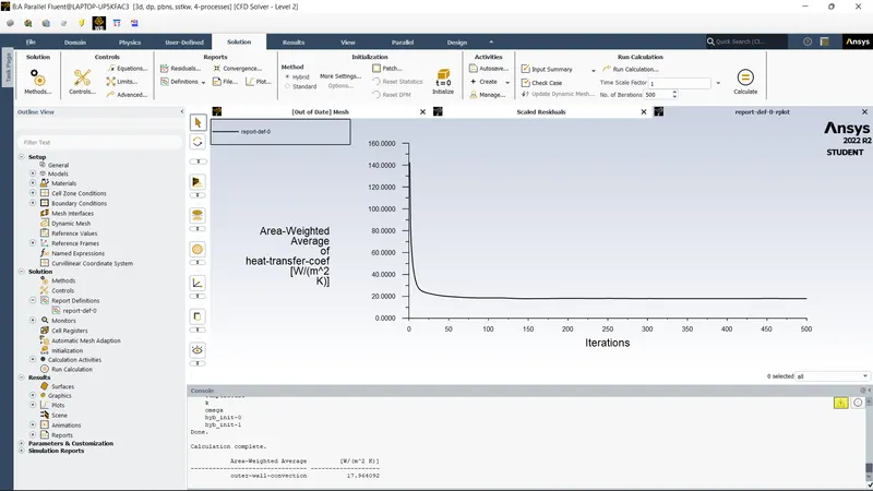
Heat Transfer coefficient
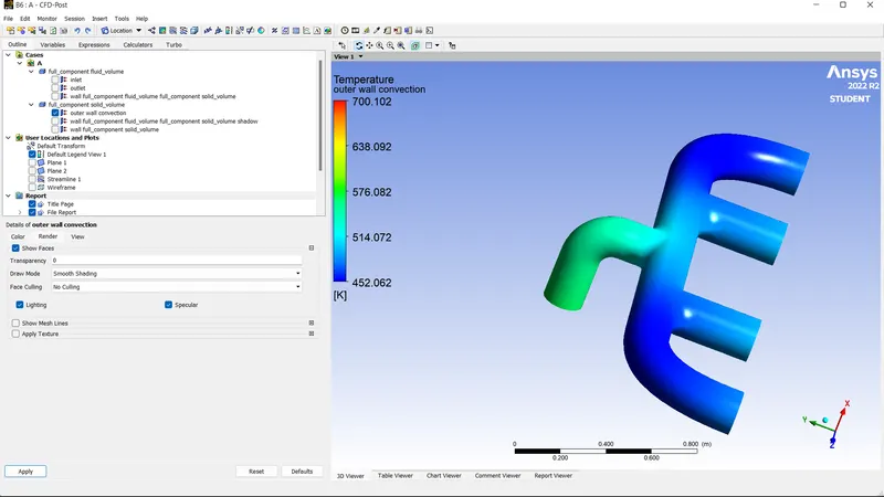
Temperature outer wall convection
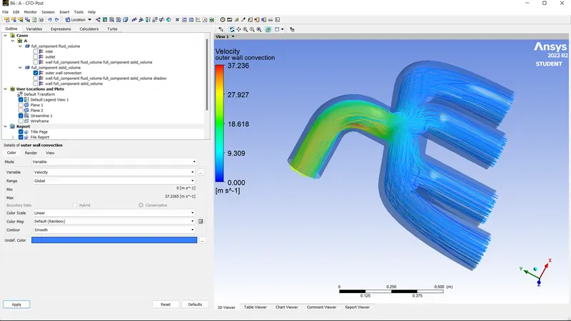
Velocity streamline
Temperature Plane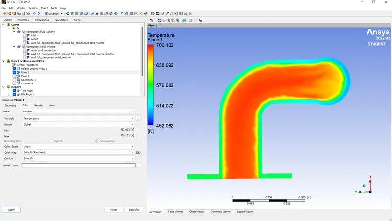
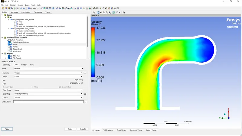
Velocity plane
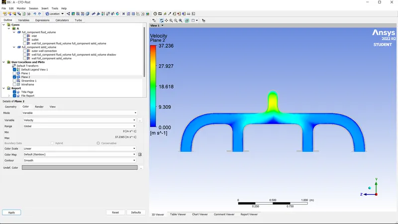
Heat transfer
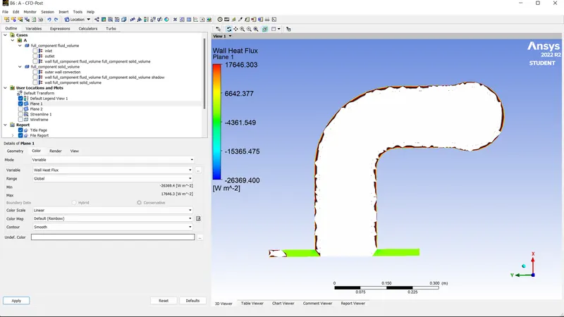
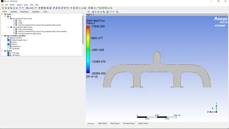
Heat transfer coefficient :

|
Heat transfer coefficient |
17.96409 |