Week 4 - CHT Analysis on Exhaust port

Aim:

To simulate an internal flow of the exhaust port and study for the Conjugate heat transfer in the simulation.

Objectives:

1. Give a brief description of why and where a CHT analysis is used.
2. Maintain the y+ value according to the turbulence model and justify the results.
   
3. Calculate the wall/surface heat transfer coefficient on the internal solid surface & show the velocity & temperature contours in appropriate areas.
4. How would you verify if the HTC predictions from the simulations are right? On what factors does the accuracy of the prediction depend on?

CHT (Conjugate heat transfer):

Conjugate heat transfer corresponds with the combination of heat transfer in solids and heat transfer in fluids. In solids, conduction often dominates whereas in fluids, convection usually dominates. Conjugate heat transfer is observed in many situations.Conduction is observed within same kind of molecules (within a solid), convection occurs between different kind of molecules where bulk motion is involved (between solid and fluid).

The Conjugate Heat Transfer (CHT) analysis type allows for the simulation of heat transfer between solid and fluid domains by exchanging thermal energy at the interfaces between them.

Conjugate Heat Transfer. In solids, conduction often dominates whereas in fluids, convection usually dominates. Conjugate heat transfer is observed in many situations. For example, heat sinks are optimized to combine heat transfer by conduction in the heat sink with the convection in the surrounding fluid.

Challenge approach:

In this challenge we have to follow five major steps Geometry, meshing, set-up, solution and result. In this challenge we have to solve two case simulation in exhaust port. We will be using ANSYS Fluent solver to create the geometry and perform unstructured tetra CFD mesh with boundary definitions. velocity of 5 m/s and k-omega SST model. Below I mentioned the two cases of element size.

Case Baseline element size (mm) Inflation layer element size (mm)

Case 1 150 150

Case 2 50 20

Step 1: Geometry

In this challenge first we have to open the geometry by using right click. Once open the geometry we have to go prepare > volume extract > select edges > click green tick symbol. So first we have to extract the volume for simulation. And then we have to give two names first one is solid volume and second one is liquid volume. And then go to workbench > share topology. Once we give the share topology the geometry process is over. After that we have to move next meshing process. In this challenge the two cases having same geometry process. So, in second case we have to the same geometry model. Nex step is meshing process.

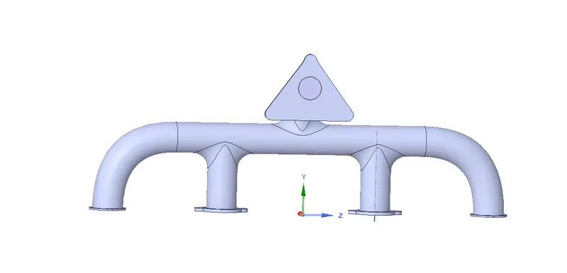
Volume exract image:

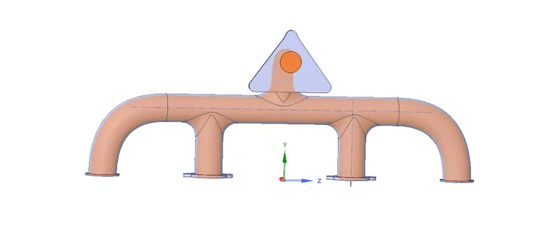
Share topology image:

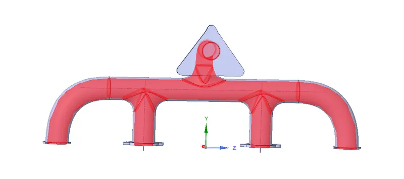
Step 2: Meshing

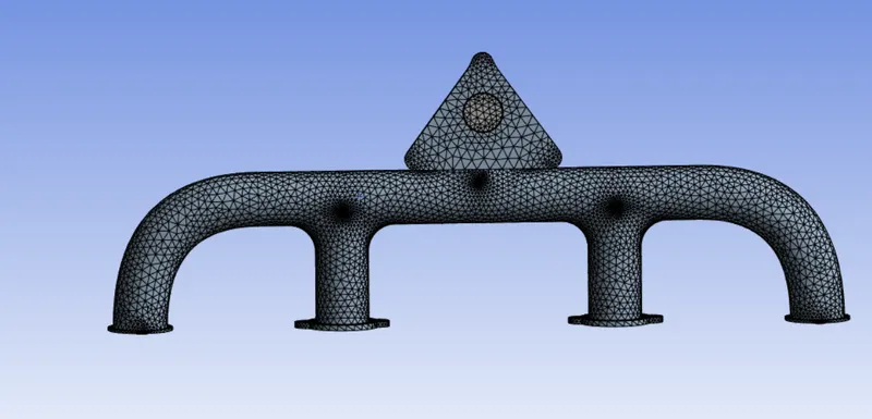
In this challenge the second step is meshing process so we have to right click on the Mesh. so, clicking on the GENERATE MESH we should create a mesh automatically. We should create INFLATION layers for the fluid volume outer surface with 0.5 mm as first layer thickness with 6 layers and 1.2 as growth factor. Since we already used share topology option, the mesh should look good. For case 1, and then go to GENERATE MESH and input size as 150 mm for inflation layer and the base mesh size shall be 150 mm. For case 2, and then go to MESH > INSERT > SIZING and input size as 50 mm for inflation layer and the base mesh size shall be 20 mm. We should give name for the geometry Inlet, Outlet, Convection Wall and inflation layer. We shall select the fluid volume outer surface and name it as inflation layer. Once we completed the meshing process after that we have to move next set-up process.

CASE 1 MESH IMAGE:

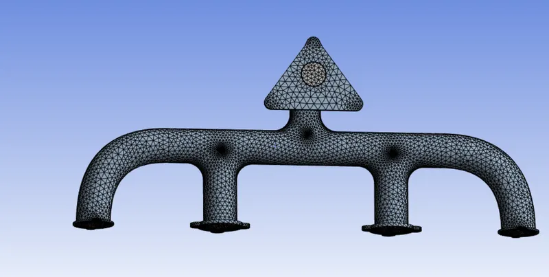
CASE 2 MESH IMAGE:

Step 3: Set-up

The third step is set-up process in this challenge so we have to right click on the Setup. we should select the Type: Pressure based, Velocity Formulation: Absolute, Time: Steady. Under the Physics tab, we can turn on viscous and select k-omega > SST as well. Turn on Energy. Method is Coupled method. And then we have selected the materials for CHT analysis, we shall consider the solid volume also with aluminium as the default solid material.

We should select the cell zone conditions, select the solid volume and check for material selection is solid, and fluid material for fluid volume. And then we have to give boundary conditions, as follows Inlet: velocity magnitude = 5 m/s, Temperature = 700 K Outlet should be a pressure outlet. For the convection wall, we can input heat transfer coefficient as 20 W/m^2 K. For generating surface reports, click on the Solution > Reports > Definitions > New > Surface Report > Area weighted average > Wall fluxes > Surface heat transfer coefficient for the heat transfer coefficient in the inflation layer.

The next step is we need to initialize the entire flow field so we have to give t=0 initialize. In the Run Calculation we can input the number of iterations to be run (in this case 150) and clicking on the Calculate should start the iterations. After iterations, we get scaled residuals, average temperature plot and standard deviation plots.

In this set-up process we need some velocity and temperature contours as well, to get them we can create a transverse cut plane i.e, XY plane and make new contour in Results > Graphics > Contours > New temperature for temperature contour and velocity for velocity contour. Once we completed the set-up process after that we have to move next solution process.

Step 4: Solution

Some solutions are completed in set-up itself. So we have move next process of the result process.

Step 5: Result

In this challenge the fifth step is result process it should open the Post processor. In the post processer the default view is a wireframe model, so we can create a plane in XY and in YZ to view contours and vectors. Selecting the Vector and selecting the plane creates a velocity vector and then create the streamline contours. For Case 2, we have to click duplicate option only we can change the mesh sizing.

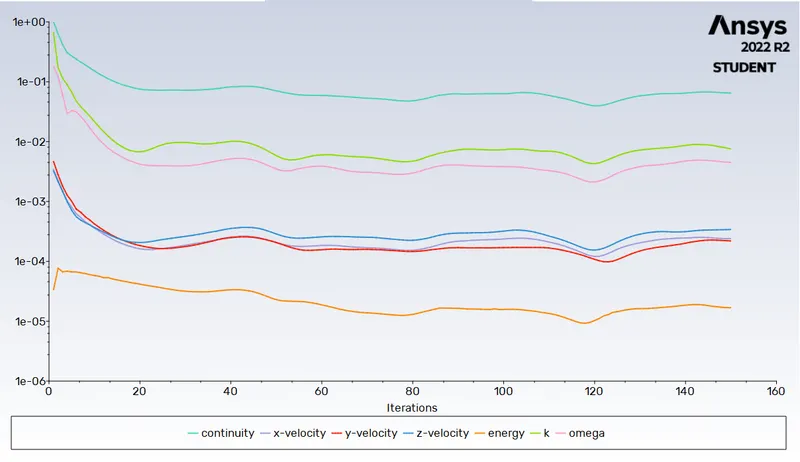
CASE 1 RESIDUAL PLOT:

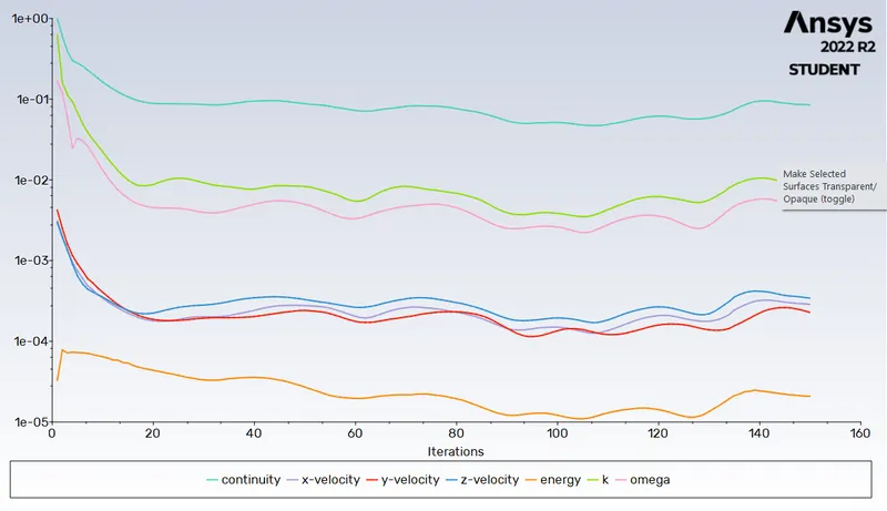
CASE 2 RESIDUAL PLOT:

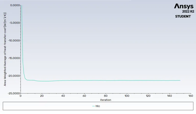
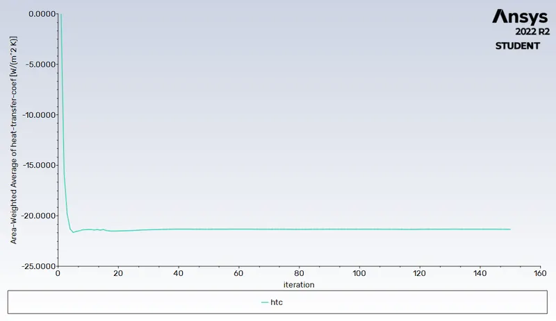
CASE 1 HTC PLOT:

CASE 2 HTC PLOT:

CASE 1 Temperature contour:

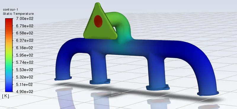
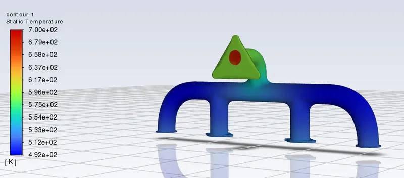
CASE 2 temperature contour:

CASE 1 velocity contour:

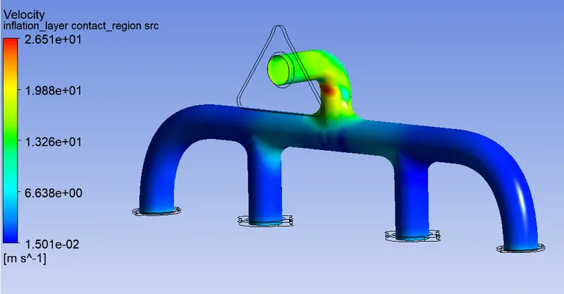
CASE 2 velocity contour:

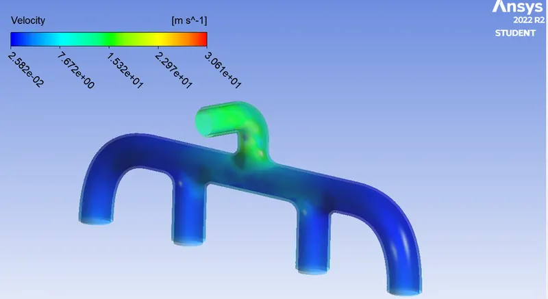
CASE 1 surface heat transfer contour:

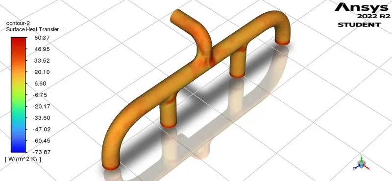
CASE 2 surface heat transfer contour:

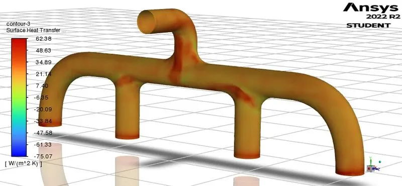
CASE 1 velocity stramline contour:

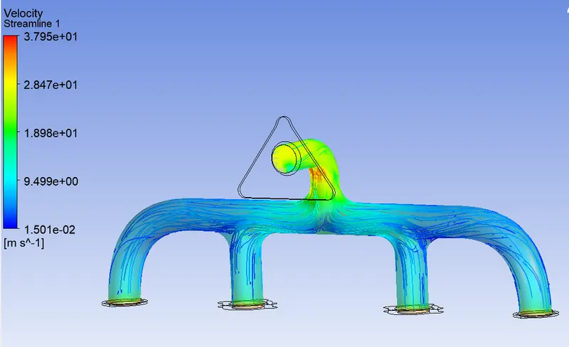
CASE 2 velocity stramline contour:

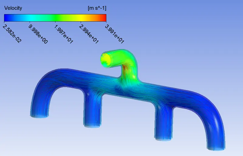
CASE 1 velocity volume rendering contour:

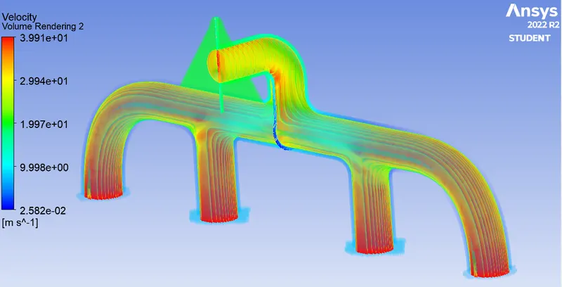
CASE 2 velocity volume rendering contour:

CASE 1 surface heat transfer coefficient contour:

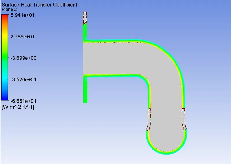
CASE 2 surface heat transfer coefficient contour:

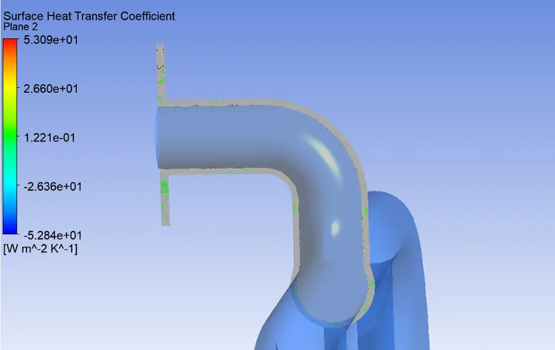
Conclusion:

Finally, we conclude the challenge, from the results of all 2 cases, we got some values for surface heat transfer coefficient with respective grid sizes.

Case 1 Case 2

Baseline mesh 150 50

Inflation layer mesh 150 20

No. of elements 242050 309852

Surface heat transfer coefficient 21.25 21.34

Inferences:

In this challenge we have to identify the grid independency study, we know that the finer and coarse mesh gives similar results. So, we have to obtained (21.3 W/m^2 K) the expected heat transfer coefficient close to 21.5 W/m^2 K. And then the finer size mesh elements don’t affect the surface heat transfer coefficient, maybe the velocity change can affect the output result. The velocity contours show wake areas at the bends. So, the surface heat transfer coefficient is higher at the bends and the inlet area, to be more specific in observation wherever the velocity is low there is increased surface heat transfer.

References:

https://www.comsol.com/blogs/conjugate-heat-transfer/#:~:text=Conjugate%20heat%20transfer%20corresponds%20with%20the%20combination%20of,Conjugate%20heat%20transfer%20is%20observed%20in%20many%20situations.