Week 4 - CHT Analysis on Exhaust port

OBJECTIVE:

The objective of this project is to perform a steady state conjugate heat transfer (CHT) analysis on an exhaust port.

Conjugate heat transfer (CHT):

Conjugate heat transfer is a type of heat transfer analysis between solids and fluids. This type of heat transfer includes both convective (between fluids) and conductive (between solids) heat transfer, as well as both forced and natural convection.

Applications:

Common applications of this thermal simulation type include electronics cooling, heat exchangers, industrial machinery, some AEC cases, and more.

Y+ concept:

This is the concept that enables us to calculate the size of the mesh element which can capture the effects of boundary layer for the given body and input parameters.

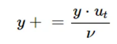
Where y+ = thickness of the first mesh element,

Y = distance from the wall.

Ut = frictional velocity,

nu = dynamic viscosity.

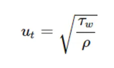
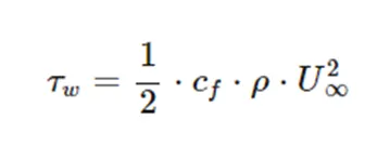
Where = wall shear stress.

Cf = skin friction coefficient.

Modelling Procedure:

1: Pre-Processing.

• Open Ansys Workbench→under Analysis system select Fluid flow(fluent) drag and drop it in Project schematic → Geometry → New spaceclaim geometry.
• File select the appropriate file and then Open the file.
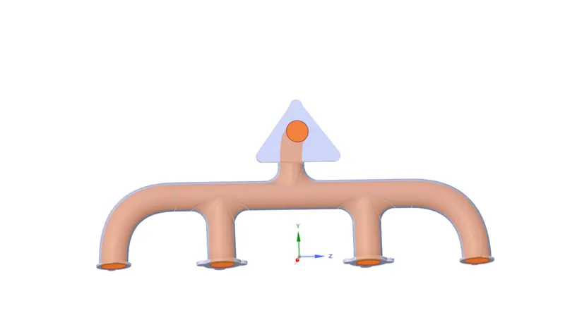
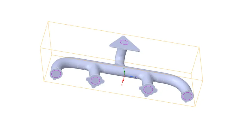
• This project is an internal flow simulation project, so we have to extract the fluid volume by using Volume extract with edge selection option in spaceclaim.
• Since we have defined a separate fluid volume from solid path, we need to share the nodes between these two bodies which will be created while meshing, to share the nodes we are using Share topology option.

Fluid volume:

Shared Topology:

2: Meshing.

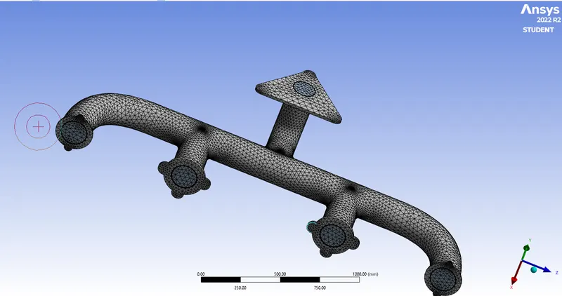
• We will proceed with mesh generation for required mesh element length using the Sizing and Inflation options. Mesh → Details of “Mesh” → Element Size then specify the required mesh length. For Inflation Inflation → Geometry select the geometry and define the inflation layer thickness and no of inflation layers.
• Then we should assign names for the parts of the geometry to make it easier while working on simulation.
• Using the y+ concept, we calculated first layer thickness as 0.5mm.

Generated Meah:

3: Simulation.

• Setting up for Physics. Choose pressure-based solver and steady state condition.
• Since we will be studying heat transfer, we should enable Energy equation option.
• The turbulence model we are using is K-omega turbulence model.
• Then define the inlet boundary conditions which is 5m/s and temperature 700k.
• Then the outlet boundary condition as Convection with heat transfer coefficient as 20 w/m^2k.
• Initialize the simulation.
• Then create the required Surface heat transfer coefficient surface plots.
• Run the simulation.

Grid Dependency test:

We have to ensure that the solution does not depend on the number of elements in the model. So, we run few simulations with different number of mesh elements. This is called Grid dependency test, where we decide the minimum number of elements required to make sure the solution is acceptable.

For the given geometry, we would run grid dependency test till we reach a point where we get solutions with acceptable error range (<0.5%). We will use the average value of drag coefficient as the parameter to obtain the ideal computational grid.

Case 1: 150mm.

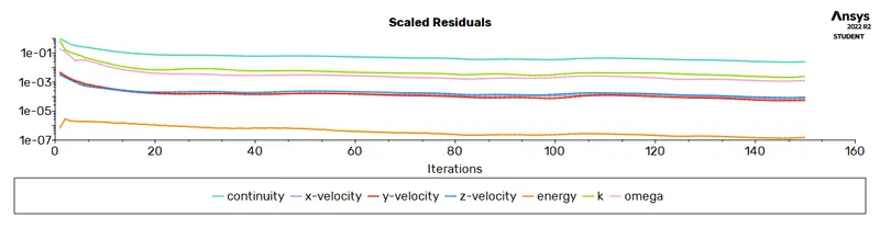
Scaled Residual:

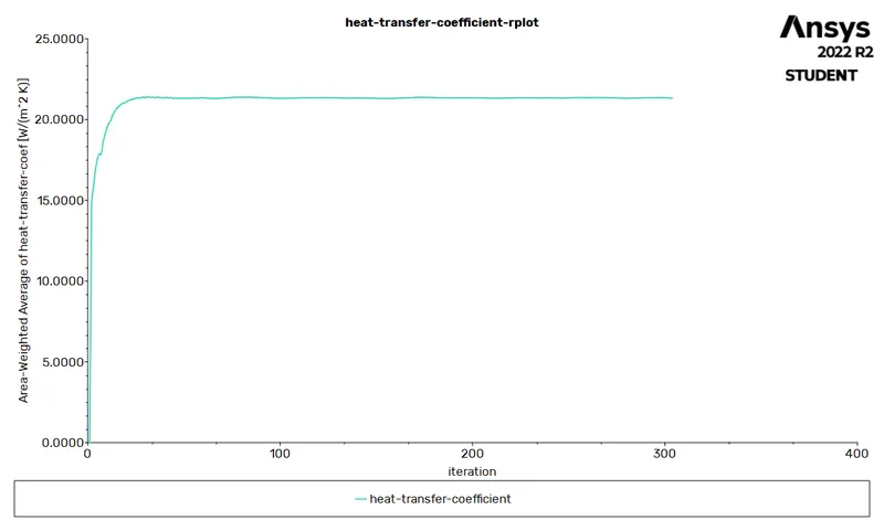
Average Heat transfer Coefficient:

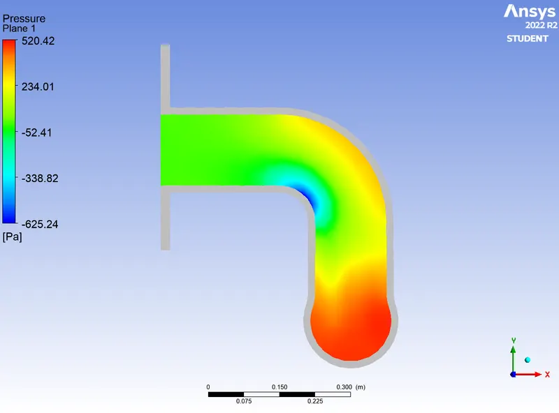
Pressure Contour:

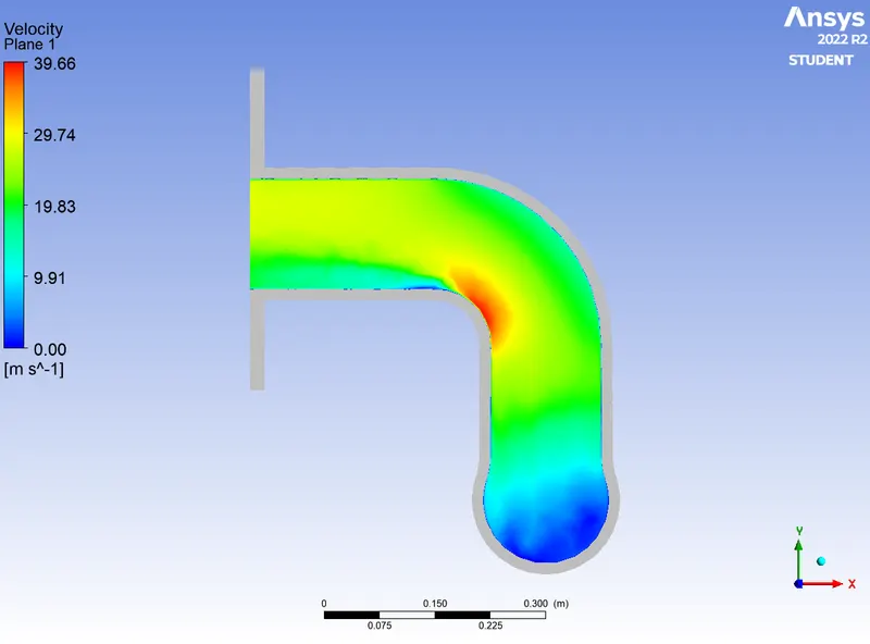
Velocity Contour:

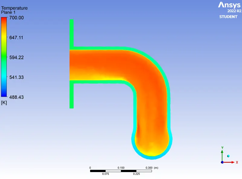
Temperature Contour:

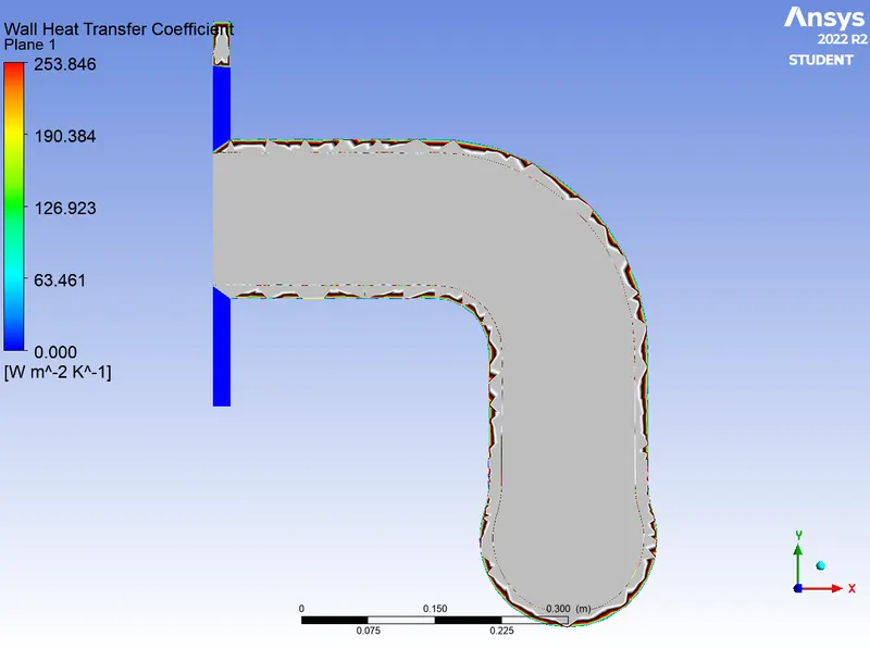
Heat transfer Coefficient:

Case 2: 75mm.

Scaled Residual:

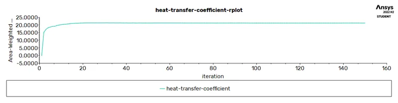
Average Heat transfer Coefficient:

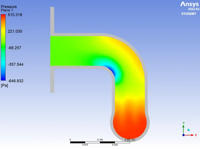
Pressure Contour:

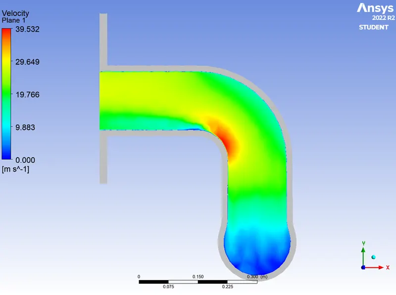
Velocity Contour:

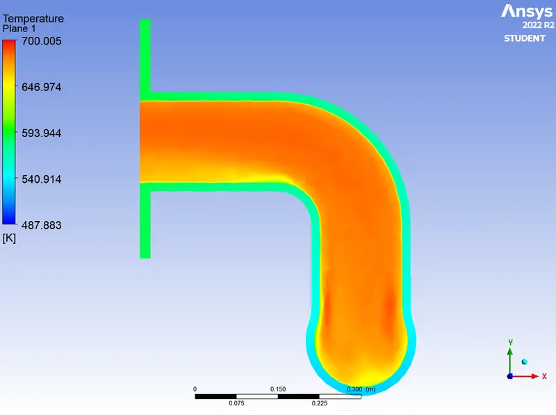
Temperature Contour:

Heat transfer Coefficient:

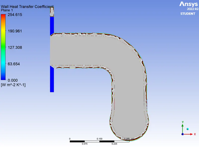
Case 3: 20mm.

Scaled Residual:

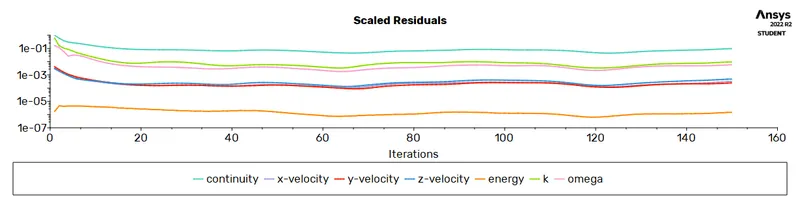
Average Heat transfer Coefficient:

Pressure Contour:

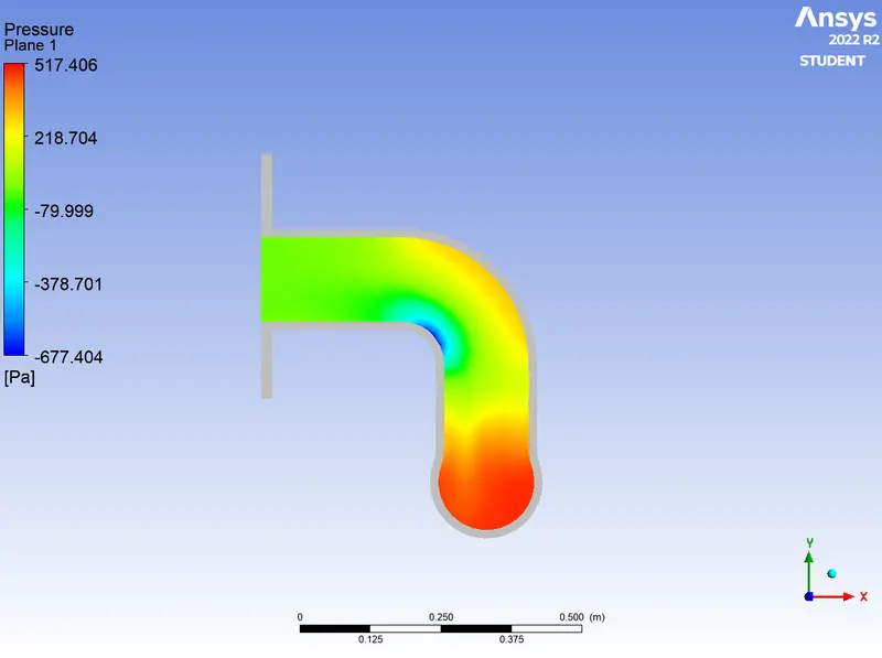
Velocity Contour:

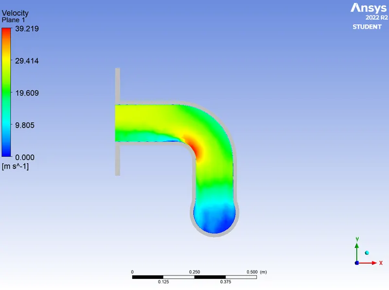
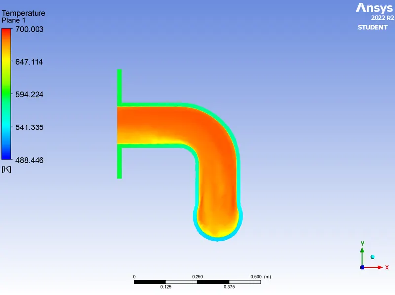
Temperature Contour:

Heat transfer Coefficient:

Analytical solution:

The input parameters of the fluid used for the calculation as follows:

Velocity at inlet (u) = 5 m/s

Density of fluid (rho) = 1.225 kg/m3

Characteristic length (d) = 0.166 m

Dynamic viscosity of fluid (mu) = 1.7894e-5 Ns/m2

Thermal conductivity (k) = 0.028 W/m K.

Specific heat (CP) = 1006.4 J/kg K.

`h=(k*Nu)/d`

where k is the thermal conductivity of the liquid,

D is the Hydraulic diameter,

Nu is the Nusselt Number which is determined by the following equation

`Nu=0.0233*Re^(4/5)*Pr^n`

n=0.4 for the fluid being heated, and n=0.3 for the fluid being cooled.

`Re=(rho*u*d)/mu=(1.225*5*0.166)/(1.7894e-5)=56820.722.`

`Pr=(mu*Cp)/k=(1.7894e-5*1006.4)/0.028=0.643.`

`Nu=0.023*(56820.7)^(0.8)*(0.643)^0.3=128.185.`

`h= (0.028*128.185)/0.166=21.622 w/(m^2k).`

Comparison:

Mesh length(mm)	No. of elements	Numerical solution`h (W/(m^2. K)) `	Error in h value%	Analytical solution`h(w/(m^2k))`	Deviation in Analytical and Numerical h value %
150	244102	21.352	-		1.24
75	255058	21.337	0.07	21.622	1.31
20	332792	21.315	0.1		1.41

Outlet Velocity Calculation:

Mass Flow rate at inlet=Mass Flow rate at outlet.

We have 4 inlets.

`4*pi/4di^2*ui=pi/4*do^2*uo`

`4*0.166^2*5=0.150^2*uo`

`uo=24.494 m/s.`

Since the value of heat transfer coefficient is nearly same for all the computational grids, we can go with the second case with element size 75mm.

The analytical value obtained for the given problem is 21.622 whereas the computational solution obtained is 21.337 W/m². K. The deviation in the value is 1.31%. Since the deviation is less than 5%, we can say the turbulence model with the given computational grid managed to capture the physics of the flow very accurately. We get the outlet velocity at outlet as 25.276 m/s. The deviation is 3.19% which is within acceptable range. Hence, the numerical solution obtained is valid.

Verify HTC :

Under forced convection circumstances, we can determine the heat transfer coefficient by using the Dittus-Boelter
correlation. Using the Dittus-Boelter correlation the heat transfer coefficient can be calculated in the following way using
two further dimensionless groups, the Reynolds number and the Prandtl number.

`Nu=0.0233*Re^(4/5)*Pr^n`

It means Nusselt no. is the function of Reynolds no. and Prandtl no.

As the turbulent boundary layer in the vicinity of bend at outlet port is thin maximum velocity of flow is observed at bend and hence higher Reynold no.As the diameter of pipe and thermal conductivity are constant, value of h will increases as Nu increases and Nu increases as Re increases.As per our results, heat transfer coefficient is high for higher value of velocity and hence from above discussion we think that our results are correct.

Factors affects the quality of prediction:

• More refined mesh leads to the better results.
• Use inflation layers and apply proper Boundary condition.
• Proper selection of turbulence model according to y+ values.

Conclusion:

The errors in the experimental and simulated values are very small. Hence, we can say the turbulence model and the computational grid captured the flow physics accurately.It is also observed at that at the bend in the pipe the velocity magnitude is maximum. This can be because of the sudden addition of the velocity components in other two co-ordinate axis. Since the velocity increases at the bends, the mass flow rate at the bend region increases, thus heat transfer coefficient at these regions also increases.