Week 4 - CHT Analysis on Exhaust port

Aim: Perform the simulation to analysis the conjugate heat transfer on exhaust port and based on mesh dependence analysing the accurate result

1. Give a brief description of why and where a CHT analysis is used?

Answer:- Conjugate heat transfer is a type of heat transfer analysis between solid and fluid this type of heat transfer includes both convective and conductive heat transfer, It used to find the convective coefficient between solids and fluid

2. Maintain the y+ value according to the turbulence model and justify the results.

Answer:-

• We know the velocity, density and viscosity by this we calculating the reynolds number by using the reynolds formula if reynold number for pipe flow greater than 4000 we consider the flow is turbulence, Based on this we use the turbulent model there is lot of turbulent model but we use major k-epsilon and k-omega model for turbulence flow cases, k-epsilon is used to capture the physics at turbulent layer and k-omega model is used to capture physics near to the wall that is at viscous sublayer, By keeping in mind which model we using based on this we calculating the yplus layer from the yplus calculator
• Yplus is the non-dimensionless layer which we calculating based on reynolds number, free stream velocity, reference length and y+models length and creating the boundary layer, Because at near the surface the fluid velocity gradient much varying so to capture the physics near to the wall fine mesh need so for this boundary layer we creating

Procedure to simulate the conjugate heat transfer analysis using exhaust port:

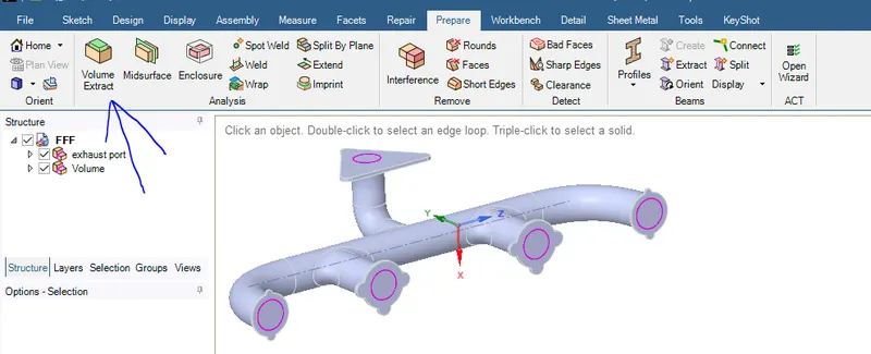
• First import geometry into the geometry space claim window, Then extract fluid volume, After give the share topology, the finished model is attached in image1
• Next open mesh window then generate mesh by giving some mesh length, Then create inflation layer but before that keeping in mind of what turbulent model we using, We calculate the first inflation layer thickness Then that criterion we give to the inflation layers this meshed model and quality criterion is shown in image2
• After mesh close mesh window open setup window, There we enable the energy equation, selecting the sst omega viscous model, Select the material for fluid and for solid, Under the cell zone condition for inside exhaust port volume select the fluid material and for the exhaust shell select solid material
• Then give the boundary condition, intialize the problem and from report under definition option take out the surface heat transfer coefficient graph sheet then run the simulation for the iteration where it will converge
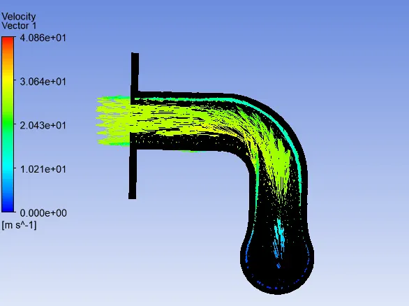
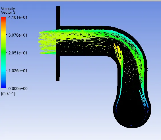
• After the calculation we taking out the contour graph for velocity by creating the plane, and taking out the pressure, Temperature contour plot as well
• In the report option under using surface integral option we taking out the result of heat transfer coefficient at the inflation and also taking out the results of (maximum/ minimum) velocity, temperature, pressure, at entire as well at the outlet position
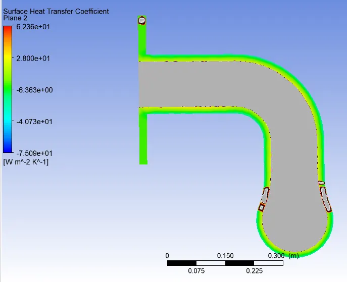
• So similarly to take out the wall surface heat transfer coefficient contour graph at the post process we export the solution data by clicking the file and select the export and click solution data option and save it in fluent file by giving file type as CDAT file, Then open post process window click on the file select load file import the data from file file where it saved So by this we read the result this result is attached in image3, image4, image5, image6
• So by this we run the simulation for two case study case1 having the mesh length of 50mm, case2 having the mesh length of 30mm

Theoritical calculation to find heat transfer coefficient:

Formula:

1. Nu = (h*D)/k

where,

Nu - Nussuelt number; D - Diameter of the pipe; k - Thermal conductivity of the material

2. Nu = 0.023*Re^0.8*Pr^0.3

where,

Re - reynolds number; Pr - prantl number

3. Reynold number = (rho*V*D)/mhu

Where,

rho - density of the fluid; V - velocity; mhu - dynamic viscosity

Calculated value:

1. Density=1.225(kg/m^3)
2. velocity=5(m/s)
3. mhu= 0.000017
4. reynolds number = 56833
5. Pr= 0.71 from data book
6. Nu= 129 from calculation
7. k=0.028 property of air
8. h= 22(W/m^2 k)

Result on the images:

First case study Result: 50mm meshed model results

Image1: Final model ready for mesh

volume extraction photo

Final model after share topology

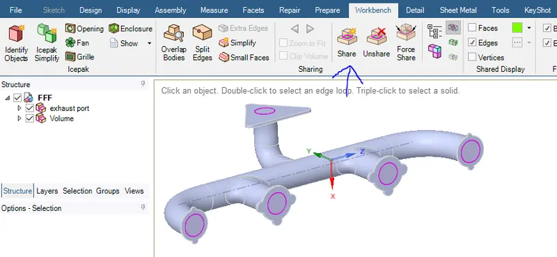
Image2 : the meshed model

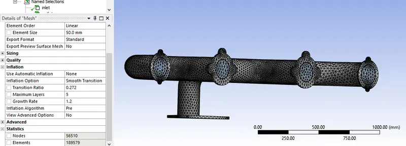
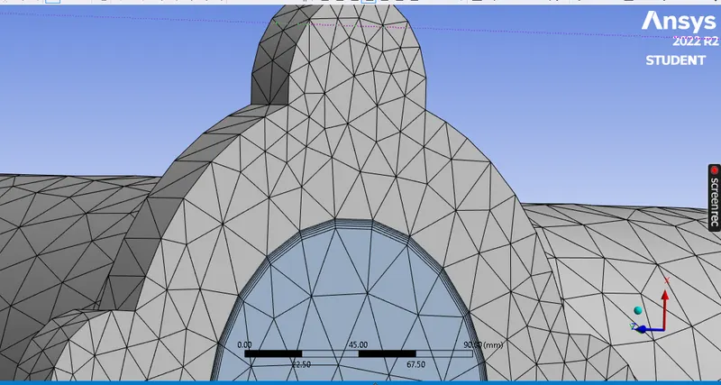
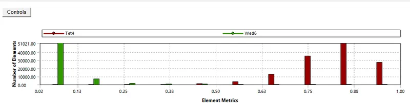
Image3: First case study scaled residual plot, area weightage averaged of heat transfer coefficient plot

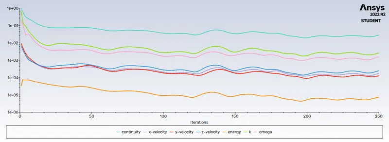
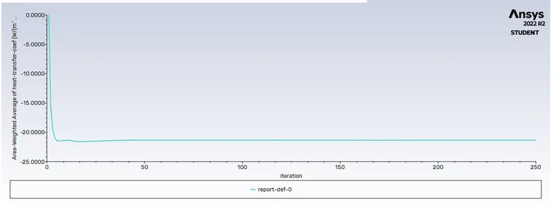
Image4: contour plot results

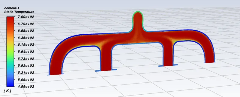
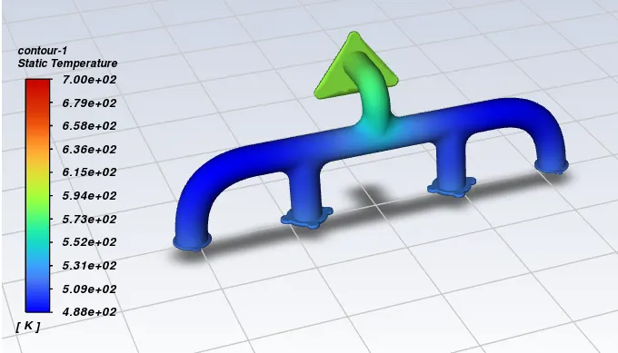
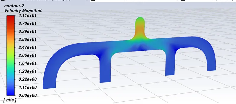
Image5: Results at the console

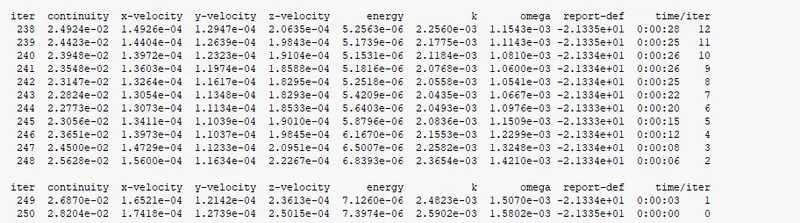
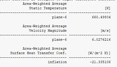
Image6: post process result

second case study Result: 30mm meshed model results

Image1: Final model ready for mesh

volume extraction photo

Final model after share topology

Image2 : the meshed model

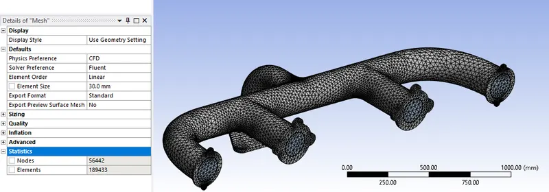
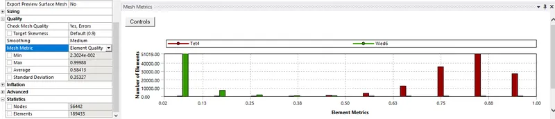
Image3: First case study scaled residual plot, area weightage averaged of heat transfer coefficient plot

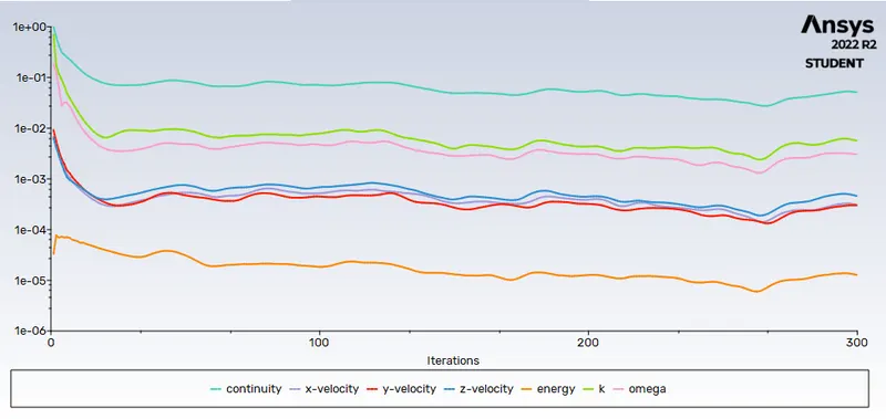
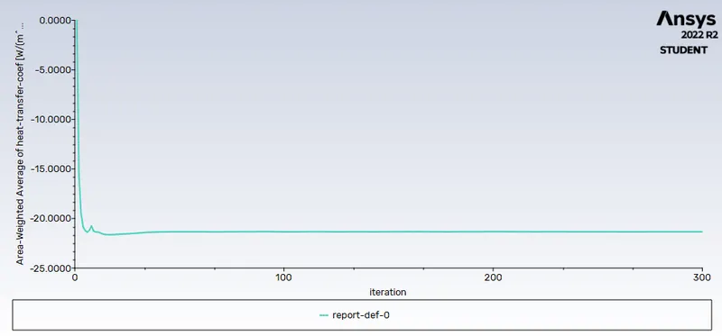
Image4: contour plot results

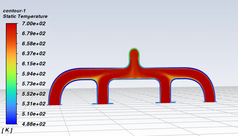
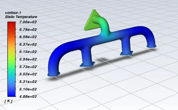
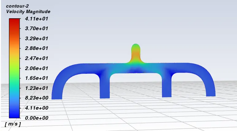
Image5: Results at the console

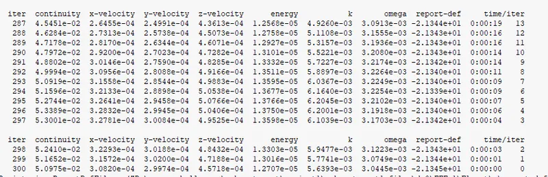
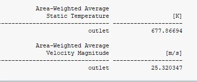
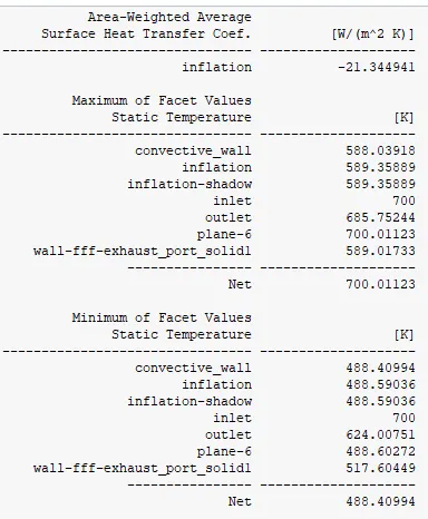
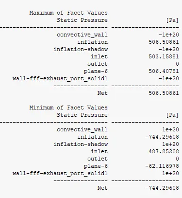
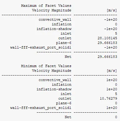
Image6: post process result

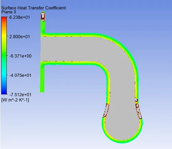
Validation : Hence by Theoritical calculation from above and simulation result matched and two case mesh gives the near similar result

Conclusion: Hence by above procedure the simulation run successfully