Week 4.1 - Genetic Algorithm

Aim: A code in MATLAB to optimise the stalagmite function and find the global maxima of the function.

Theory :

• In matlab to find the global maxima of function the inbuilt solver helps that is 'ga'
• Generally the 'ga' is genetic allgorithm this mainly based on ideology of charles darwin

Genetic allgorithm:

1. It is inbuilt solver in matlab that finds the minimum of function.
2. There are three syntax using in this code that is

synatax 1: x = ga(fun,nvars)

This syntax says that taking 2 inputs and used in function that function is minimize by inbuilt solver that is 'ga'(genetic allgorithm)

syntax 2 : x = ga(fun,nvars,A,b,Aeq,beq,lb,ub)

• In starting of program we defining the inputs that is x variable and y variable but it doesn't define searchspace for genetic allgorithm but we want searchspace
• Means that genetic allgorithm doesn't know that range of given x and y variable value going to be beyond the limit or going to below the limit so that's why in this sytax we giving lower bound and upper bound but A, b ,Aeq, beq are constant this constat we keep as null matrix in the code

syntax 3 : x = ga(fun,nvars,A,b,Aeq,beq,lb,ub,nonlcon,intcon,options)

• By using above syntax 1 and syntax 2 writing code finds local maxima of the function
• So there is inbuilt in matlab that is optimization by this we actually going to finds global maxima of the function by giving number of population
• so this population optimization send to syntax 3 that is shown in syntax 3 in last of syntax options given this is taking population optimization and gentic allgorithm solves this and gives minimum of function

Code explanation:

1.Below image is the main code:

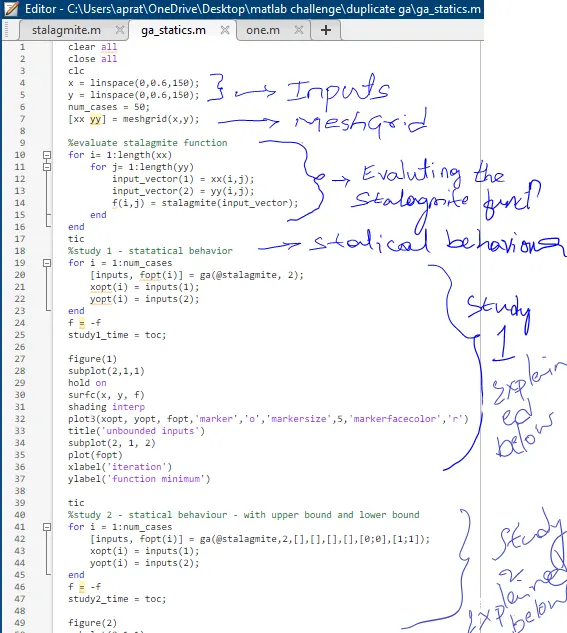
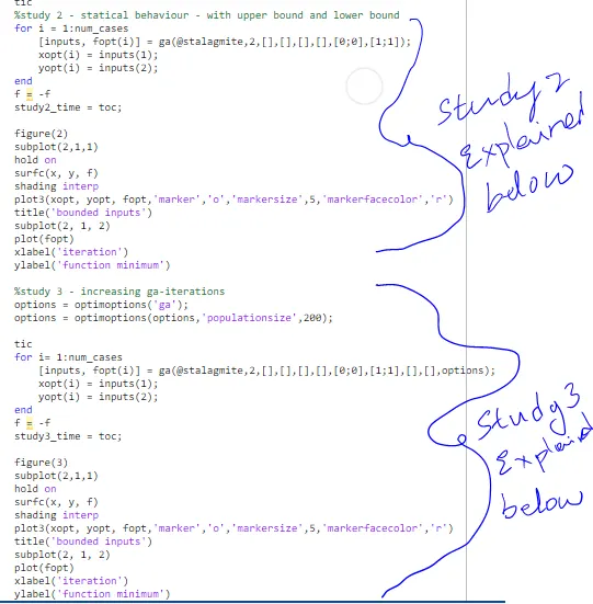
• In above code we giving input of x and y value first then it is meshgrid using matlab solver meshgrid
• then giving input to variable that is to the num_cases that says how much iteration that stalagmite function to run
• Then we are evaluating the the stalagmite function
• Then we are studying three cases studies that is

1. study-1: statatical behaviour without unbounded
2. study-2: statatical behaviour with bounded
3. study-3: increasing ga-iteration

Study-1:

• In first study that the code says that my genetic allgorithm executes with number of iteration (which mention in num_cases)using for loop
• But the genetic allgorithm doesn't know that given value in the x and y value going to beyond or below the limit so we are going study to another case that is study-2

Study-2

• In this case we know that sytax-2 using this genetic allgorithm know the searchspace that my value that x and y value going beyond limit and below the limit
• But this is showing local minimum of the function but to know global minimum of the function study case 3 there which give exact genetic allgorithm

study-3

• In this we using matlab inbuilt solver that is optimoption which optimize by number of population which mention
• hence that option mention in sytax-3 that gives global optimotion

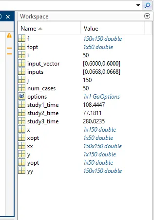
But to run this it take time that mention using tic, toc as shown in program and also before the study_time we providing f=-f this gives maxima of function

Ploting of graph:

• After each case study we ploting graph that shows comparision how smoother last graph than other graph
• But in sigle sheet plotting two graph we are using subplot as shown in program

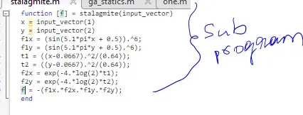
2.But to call stalagmite function sub program is to write Below is the sub program:

output of the program:

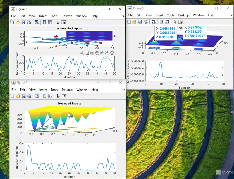
codes:

1.main code:

clear all
close all
clc
x = linspace(0,0.6,150);
y = linspace(0,0.6,150);
num_cases = 50;
[xx yy] = meshgrid(x,y);

%evaluate stalagmite function
for i= 1:length(xx)
    for j= 1:length(yy)
        input_vector(1) = xx(i,j);
        input_vector(2) = yy(i,j);
        f(i,j) = stalagmite(input_vector);
    end
end
tic
%study 1 - statatical behavior
for i = 1:num_cases
    [inputs, fopt(i)] = ga(@stalagmite, 2);
    xopt(i) = inputs(1);
    yopt(i) = inputs(2);
end
f = -f
study1_time = toc;

figure(1)
subplot(2,1,1)
hold on
surfc(x, y, f)
shading interp
plot3(xopt, yopt, fopt,'marker','o','markersize',5,'markerfacecolor','r')
title('unbounded inputs')
subplot(2, 1, 2)
plot(fopt)
xlabel('iteration')
ylabel('function minimum')

tic
%study 2 - statical behaviour - with upper bound and lower bound
for i = 1:num_cases
    [inputs, fopt(i)] = ga(@stalagmite,2,[],[],[],[],[0;0],[1;1]);
    xopt(i) = inputs(1);
    yopt(i) = inputs(2);
end
f = -f
study2_time = toc;

figure(2)
subplot(2,1,1)
hold on
surfc(x, y, f)
shading interp
plot3(xopt, yopt, fopt,'marker','o','markersize',5,'markerfacecolor','r')
title('bounded inputs')
subplot(2, 1, 2)
plot(fopt)
xlabel('iteration')
ylabel('function minimum')

%study 3 - increasing ga-iterations
options = optimoptions('ga');
options = optimoptions(options,'populationsize',200);

tic
for i= 1:num_cases
    [inputs, fopt(i)] = ga(@stalagmite,2,[],[],[],[],[0;0],[1;1],[],[],options);
    xopt(i) = inputs(1);
    yopt(i) = inputs(2);
end
f = -f
study3_time = toc;

figure(3)
subplot(2,1,1)
hold on
surfc(x, y, f)
shading interp
plot3(xopt, yopt, fopt,'marker','o','markersize',5,'markerfacecolor','r')
title('bounded inputs')
subplot(2, 1, 2)
plot(fopt)
xlabel('iteration')
ylabel('function minimum')

2.sub program:

function [f] = stalagmite(input_vector)
x = input_vector(1)
y = input_vector(2)
f1x = (sin(5.1*pi*x + 0.5)).^6;
f1y = (sin(5.1*pi*y + 0.5).^6);
t1 = ((x-0.0667).^2/(0.64));
t2 = ((y-0.0667).^2/(0.64));
f2x = exp(-4.*log(2)*t1);
f2y = exp(-4.*log(2)*t2);
f = -(f1x.*f2x.*f1y.*f2y);
end