Week 3 - Solving second order ODEs

Aim: Program in Matlab that will simulate the pendulum motion

Theory:

In Engineering, ODE is used to describe the transient behavior of a system. A simple example is a pendulum

The way the pendulum moves depends on the Newtons second law. When this law is written down, we get a second order Ordinary Differential Equation that describes the position of the "ball" w.r.t time.

This equation when integrate with respect to time we find the position of pendulum with velocity at particular time when it disturb

Code explanation and ode solver inbuilt explantion:

• In above equation b,m,g,l are paramter
• This parameter value is given as input
• then give input of initial theta and velocity value in form of matrix
• Then using ode solver inbuilt function integrating above equation by calling the function this is shown in below program
• the above equation that is differentiating term is given in other function
• after to plot the pendulum for loop is used
• In for loop theta changing range is given
• Then first and last location of simple pendulum coordinates are given that is shown in below

x0= 0;

y0= 0;

x1 = l*sin(result(i,1));

y1 = -l*cos(result(i,1));

• Then using plot command plotting horizontal line by giving intial x value and final x value putting intial and final y value zero
• Then use hold on command to plot the pendulum oscillation in same graph
• And again use plot command and give above coordinates that is x0,y0,x1,y1 so it's tells that pendulum oscillates with respect to time theta changing
• Then once again use plot command give x1 y1 coordinate next give 'o'and give marker size tells that pendulum ball locating at that point
• atlast use pause that tell how much time the video will be
• Then m(ct) = getframe(gcf) is used to store the video
• next give ct = ct+1 to repeat for loop and also to note that before giving for loop ct intial value to store that is ct=1 then end given to end the for loop
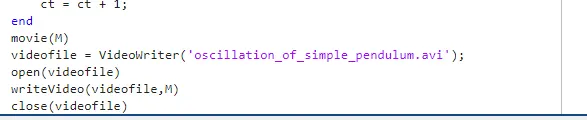
• By this video movie is creating by using below command

movie(M)

videofile = VideoWriter('oscillation_of_simple_pendulum.avi');

open(videofile)

writeVideo(videofile,M)

close(videofile)

ODE solver in built function explanation:

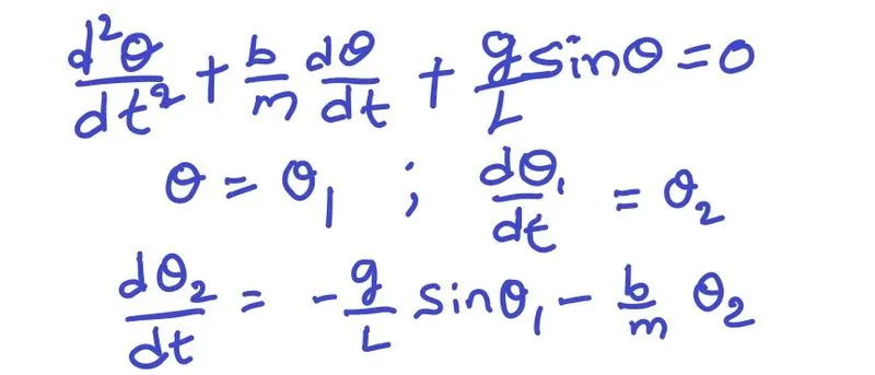
ODE inbuilt is the solver by integrating solve the first order derivative so in above equation it is not first order equation so that's why first we converting higher order into first order as shown in below picture

Below is the program run in matlab:

1st program

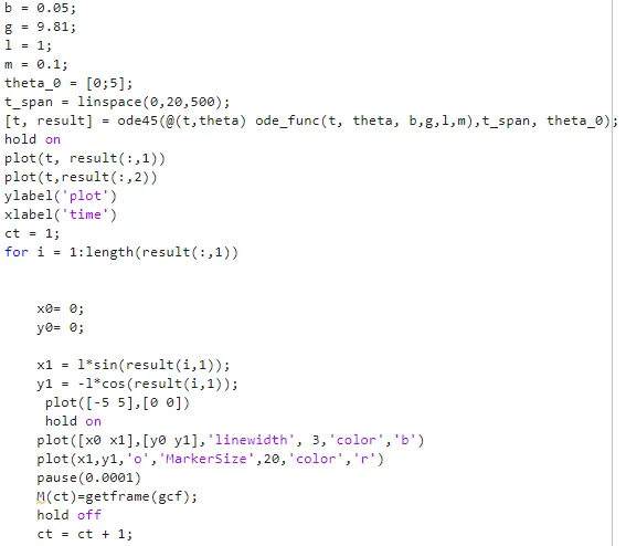
2nd program

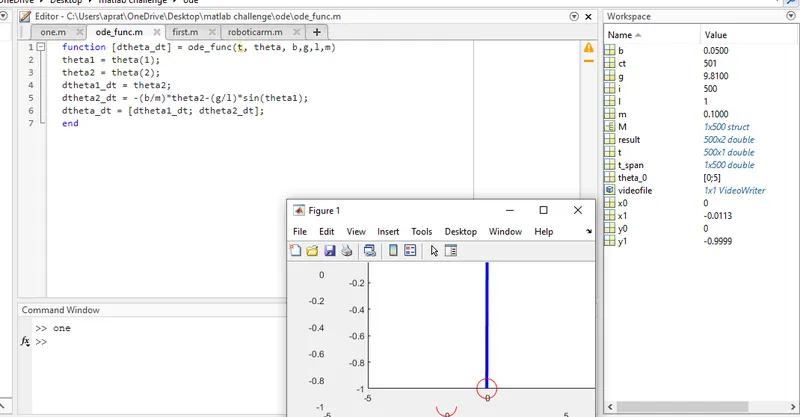
link of simple pendulum oscillation animation: https://drive.google.com/file/d/1kRhumwhzhDw4ukx6dohKHbKMKD18zkdX/view

Program:

1. main program

b = 0.05;
g = 9.81;
l = 1;
m = 0.1;
theta_0 = [0;5];
t_span = linspace(0,20,500);
[t, result] = ode45(@(t,theta) ode_func(t, theta, b,g,l,m),t_span, theta_0);
hold on
plot(t, result(:,1))
plot(t,result(:,2))
ylabel('plot')
xlabel('time')
ct = 1;
for i = 1:length(result(:,1))
    
   
    x0= 0;
    y0= 0;
   
    x1 = l*sin(result(i,1));
    y1 = -l*cos(result(i,1));
     plot([-5 5],[0 0])
     hold on
    plot([x0 x1],[y0 y1],'linewidth', 3,'color','b')
    plot(x1,y1,'o','MarkerSize',20,'color','r')
    pause(0.0001)
    M(ct)=getframe(gcf);
    hold off
    ct = ct + 1;
end
movie(M)
videofile = VideoWriter('oscillation_of_simple_pendulum.avi');
open(videofile)
writeVideo(videofile,M)
close(videofile)

2.funtion program

function [dtheta_dt] = ode_func(t, theta, b,g,l,m)
theta1 = theta(1);
theta2 = theta(2);
dtheta1_dt = theta2;
dtheta2_dt = -(b/m)*theta2-(g/l)*sin(theta1);
dtheta_dt = [dtheta1_dt; dtheta2_dt];
end