Week 4 - CHT Analysis on Exhaust port

CHT Analysis on Exhaust port

AIM:-

• To perform and study Conjugate Heat Transfer (CHT) analysis on the Exhaust Port model.

OBJECTIVES:-

1. Give a brief description of why and where a CHT analysis is used.
2. Maintain the y+ value according to the turbulence model and justify the results.
3. Calculate the surface heat transfer coefficient on the internal solid surface & show the velocity & temperature contours in appropriate areas.
4. Verify the HTC predictions from the simulations are correct.

THEORY:-

The Conjugate Heat Transfer (CHT) analysis allows for the simulation of heat transfer between solid and fluid domains by exchanging thermal energy at the interfaces between them. Typical applications of this analysis type exist as, but are not limited to, the simulation of heat exchangers, cooling of electronic equipment, and general-purpose cooling and heating systems.

CHT analysis can accurately predict heat transfer by simultaneously solving all the relevant solid and flow domain heat transfer processes, for e.g, conduction through solids, free and forced convection in the gases/fluids, and thermal radiation. The CHT approach has an advantage over Finite Element Thermal analysis in that wall heat transfer coefficients and their local variations on surfaces are directly calculated within the model rather than based on simplified empirical calculations. The CHT approach, therefore, has benefits for these applications where heat transfer is either non-uniform or difficult to calculate empirically.

Heat Transfer coefficient

The heat transfer coefficient is a quantitative characteristic of convective heat transfer between a fluid medium (a fluid) and the surface (wall) flowed over by the fluid.

The general definition of the heat transfer coefficient is:

where:

q = heat flux, W/m²; i.e., thermal power per unit area,

h = heat transfer coefficient, W/(m²K)

ΔT = difference in temperature between the solid surface and surrounding fluid area, K

Experimental assessment of the heat transfer coefficient poses some challenges especially when small fluxes are to be measured.

MODELING APPROACH:-

• A model containing 4 inlet ports and a single outlet port is considered.
• The conjugate heat transfer analysis is conducted to find the average surface heat transfer coefficient.
• Fluid volume is extracted from the port and considered as the fluid domain where the air (fluid) enters.
• Here we consider the solid domain as we are studying the combined effect of conduction and convection.

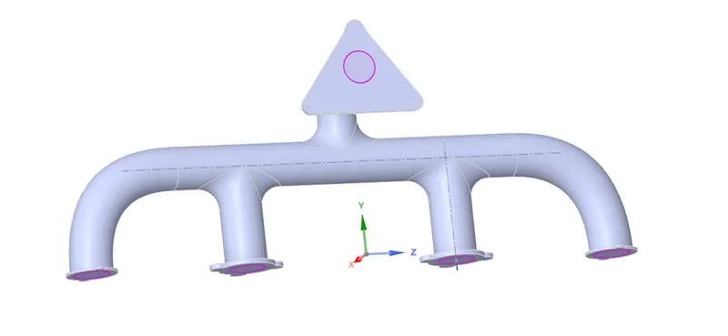
PREPROCESSING

Geometry:-

• Import the model into SpaceClaim and change the units into meters.
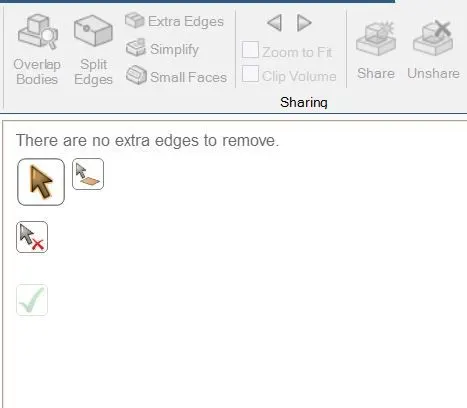
• Remove the extra edges present. For that Workbench ⇒ Extra edges ⇒ click Ok. The software will auto-detect any extra edges. The extra edges should be removed in order to perform volume extraction.

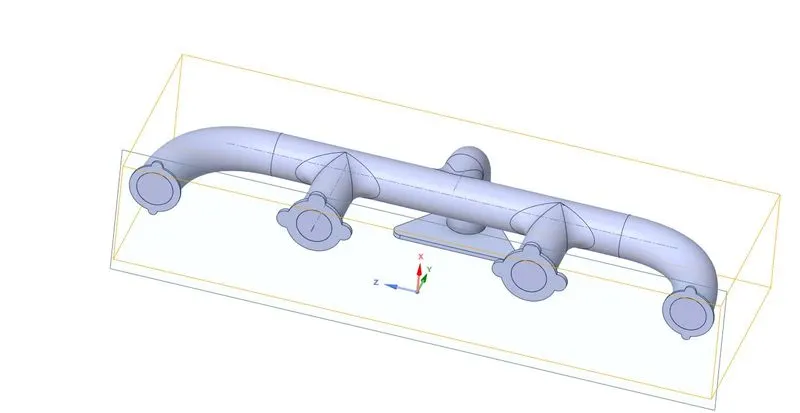
• Extract the fluid volume using the Volume Extract tool. For that Prepare ⇒ Volume extract ⇒ select edge mode ⇒ click the edges needed for separation ⇒ click Ok.

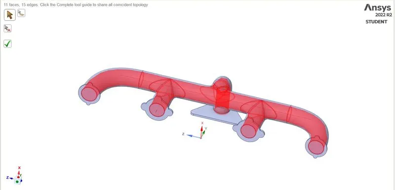
• Use the Share tool which is available in the Workbench for sharing the topology. This will create common nodes for both solid and fluid domains while generating mesh.

Meshing:

• Open the Mesh window and use 'Generate mesh' to mesh the geometry (element size - 150mm).
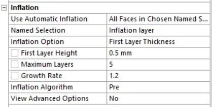
• Add inflation layers maintaining the y+ value according to the turbulence model.

Name selection – Inflation Layer

Inflation option – First Layer Thickness

First layer height – 0.05 mm

Maximum layers – 5

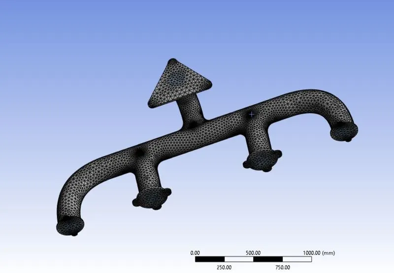
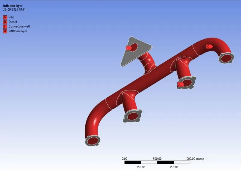
• Name the boundaries as inlet, outlet, Convective wall, and inflation layer. The inflation layer is the outer layer of the fluid volume.

• For cases 2 and 3, we will reduce the element size to 50mm and 20mm respectively.

Setup:

Fluent Setup

1.	Solver Type	Pressure based
2.	Solver Time	Steady-state
3.	Energy	ON
4.	Turbulence model	k omega SST
5.	Material	Air
6.	Inlet	Velocity Inlet (5 m/s) Temperature - 700K
7.	Outlet	Pressure outlet
8.	Convective Wall	Wall - convection - 20 W/m2K
9.	Internal solid surface	Wall BC
10.	Method	Coupled

• Create a report for Surface heat transfer coefficient.

• Create a contour for the temperature to analyze the temperature distribution.

• Run the simulation for 150 iterations after performing the Hybrid initialization

• The setup remains the same for cases 2 and 3.

RESULTS

Case 1 (Element size - 150mm)

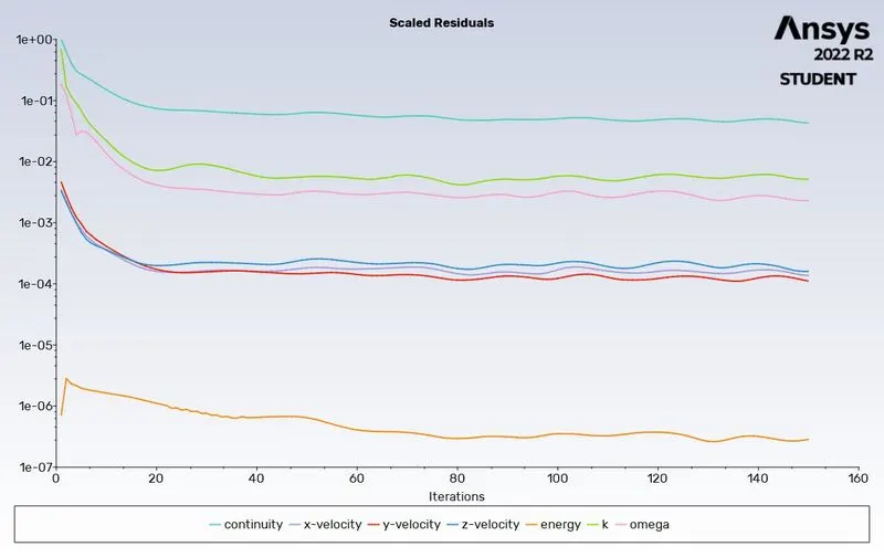
• Residual plot

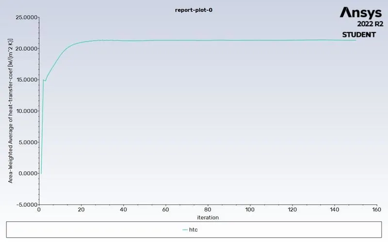
• Surface heat transfer coefficient

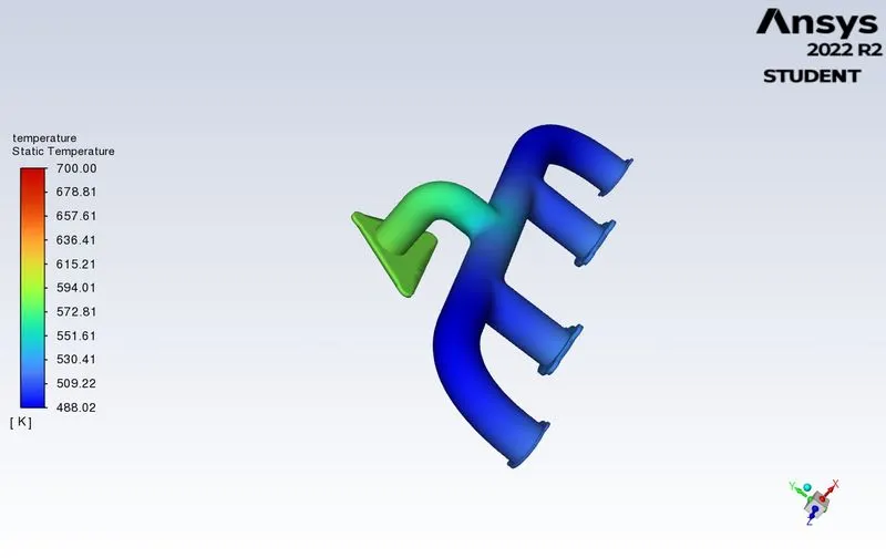
• Temperature contour

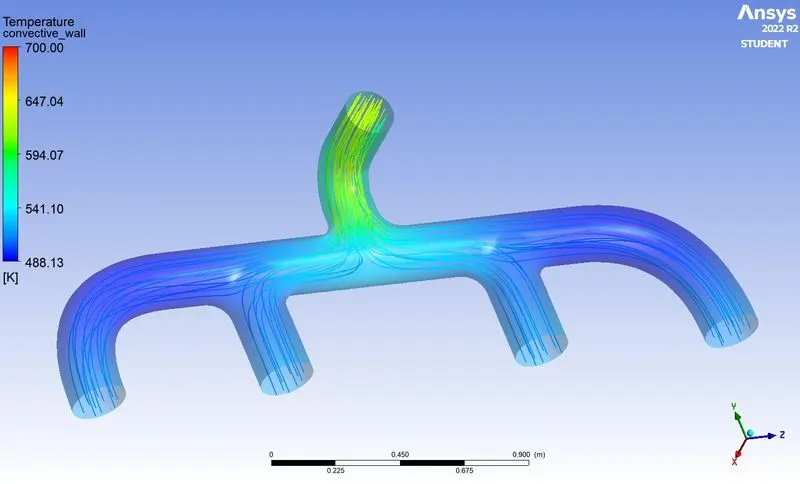
• Velocity Streamlines

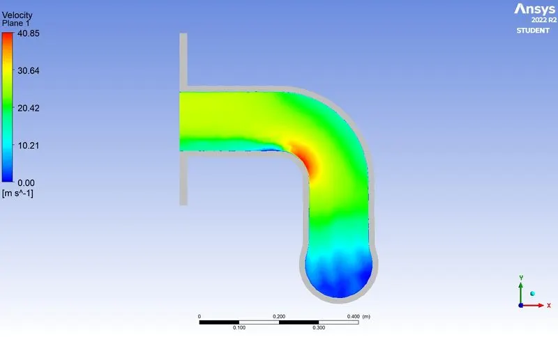
• Velocity contour

• Pressure contour

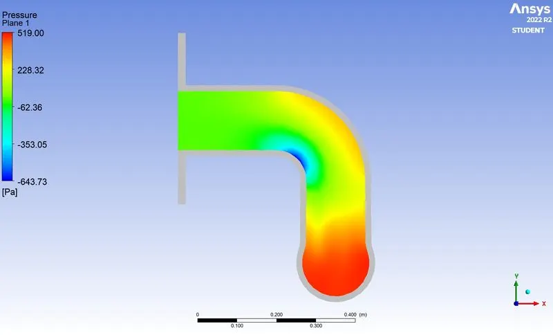
• Surface heat transfer coefficient

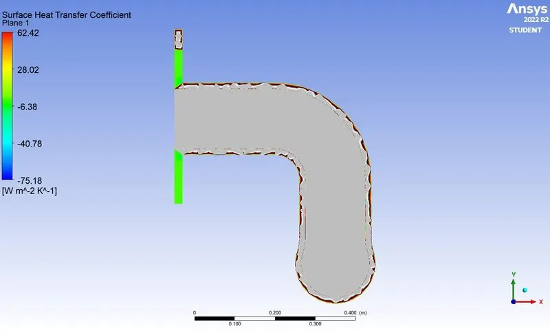
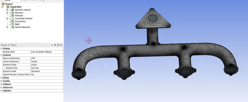
Case 2 (Element size - 50mm)

• Refined mesh

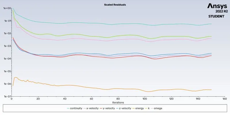
• Residual plot

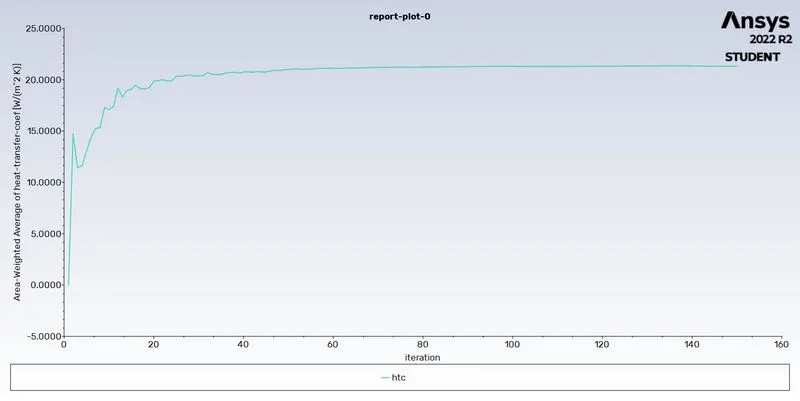
• Surface heat transfer coefficient

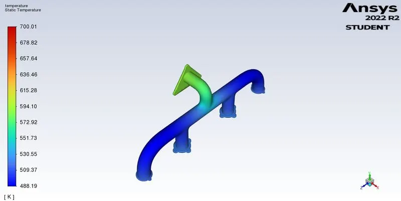
• Temperature contour

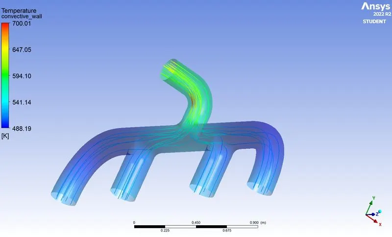
• Streamlines

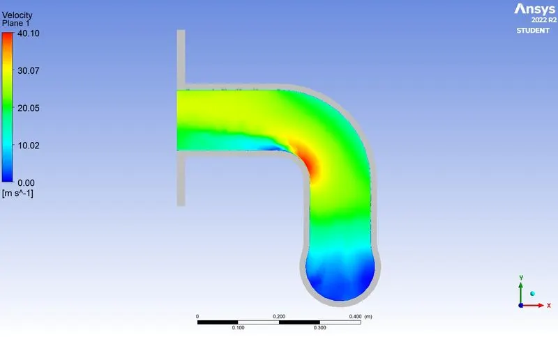
• Velocity contour

• Pressure contour

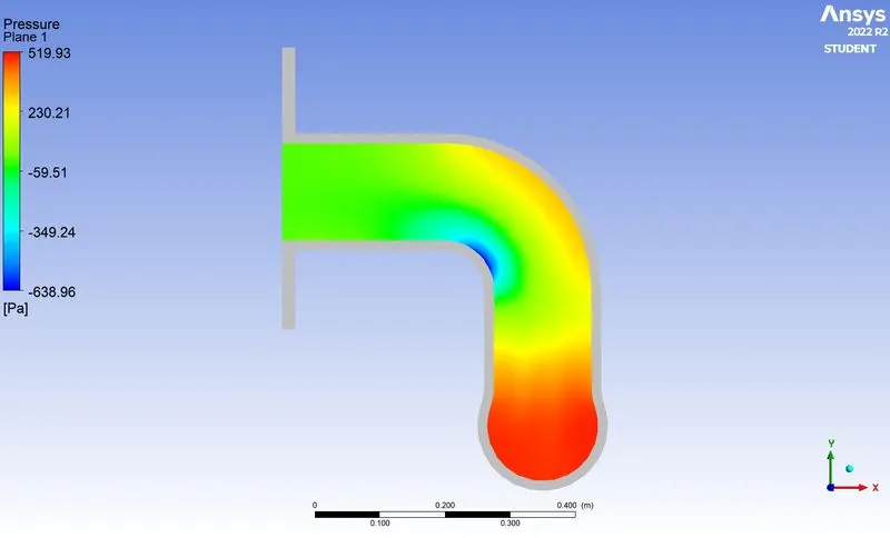
• Surface heat transfer coefficient

Case 3 (Element size - 20mm)

• Refined mesh

• Residual plot

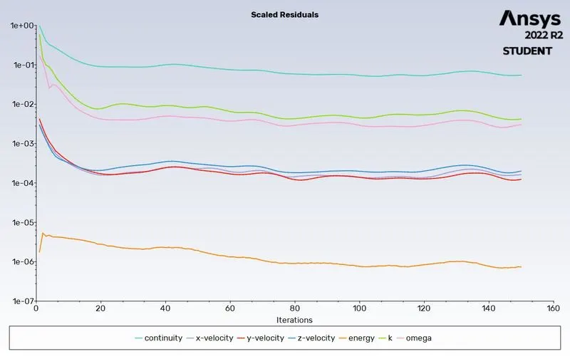
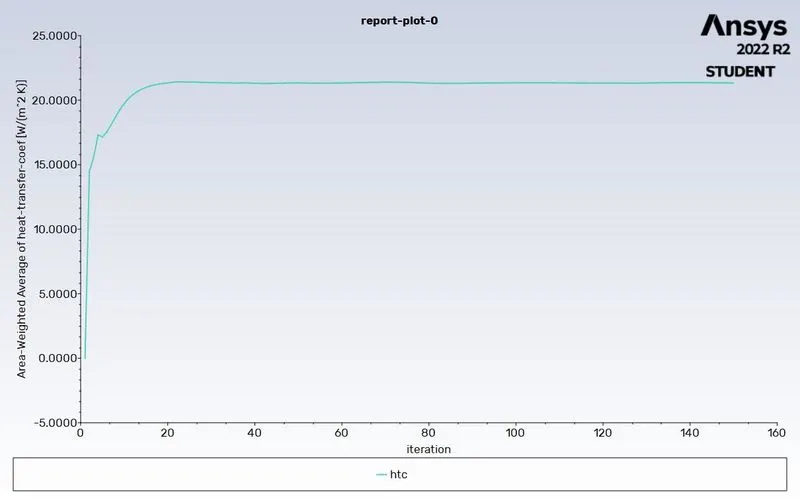
• Surface heat transfer coefficient

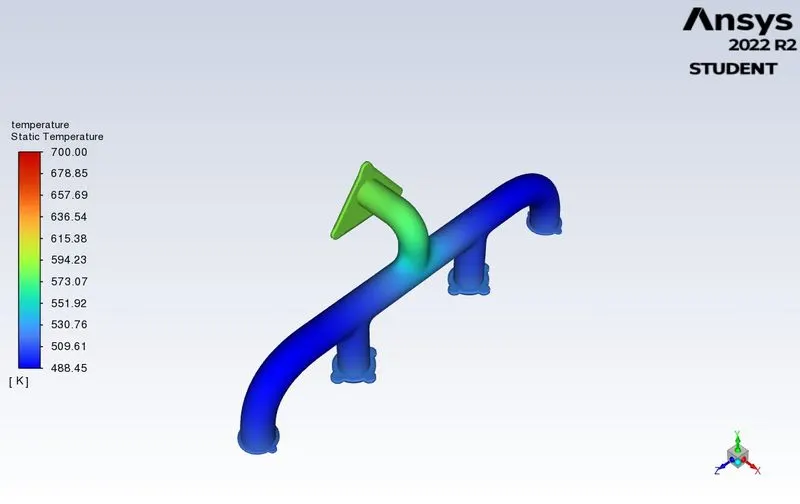
• Temperature contour

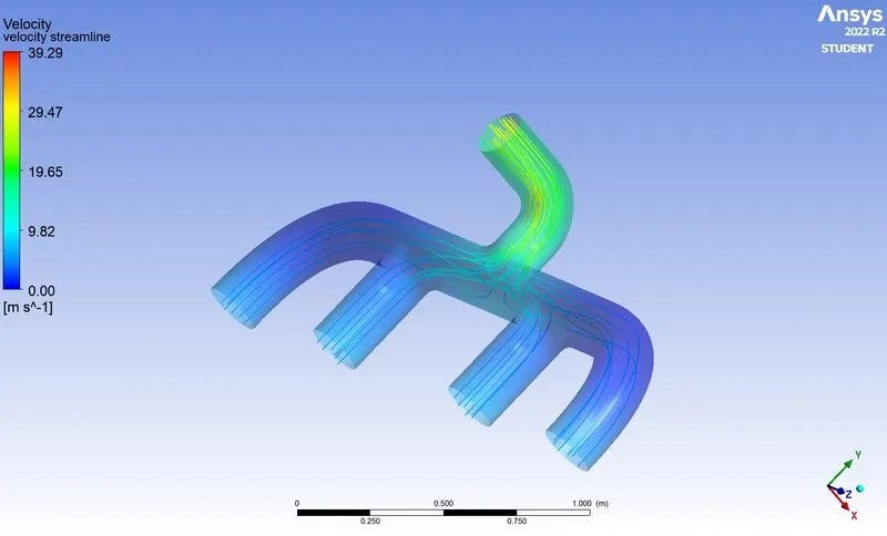
• Streamlines

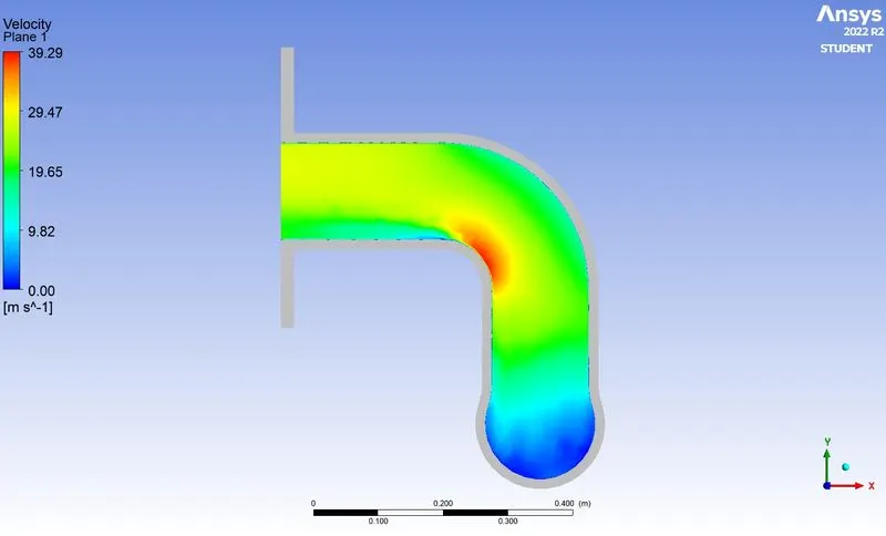
• Velocity contour

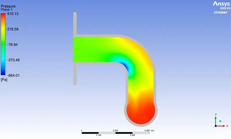
• Pressure contour

• Surface heat transfer coefficient

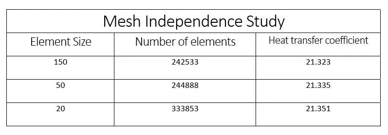
Observations

CONCLUSION:

1. The CHT analysis on the given geometry was simulated successfully on Ansys-fluent.
2. The velocity at the outlet is higher than the velocity at the inlet. This can be explained using the law of conservation of mass. There are 4 inlets and a single outlet.
3. From the velocity and temperature contours, we can see the region where the velocity is high. Because of that high velocity, the Re number will be higher which results in a higher value of the heat transfer coefficient. This area will have a higher rate of heat transfer coefficient.
4. Surface heat transfer coefficient values remained almost the same even after refining the mesh. As there is a limit of 5 lakh elements, only 3 cases were discussed here. From this, we can infer that the default mesh size of 150mm is enough so that computational time can be saved.
5. The value of the heat transfer coefficient from the analytical method was 23.76 W/m2K. This is almost equal to the value from numerical methods.
6. The accuracy of the heat transfer coefficient depends on selecting the suitable value of y+ and turbulence model K-omega SST model.

REFERENCES

1. https://volupe.se/wall-y-calculator-when-meshing-a-geometry-for-cfd-analysis-this-handy-volupe-calculator-computes-the-height-of-the-first-mesh-cell-off-the-wall-required-to-achieve-a-desired-y-using-flat-plate-boun/
2. https://www.thermopedia.com/content/841/
3. https://www.simscale.com/docs/analysis-types/conjugate-heat-transfer-analysis/