Week 4 - CHT Analysis on Exhaust port

Objective: To perform Conjugate Heat Transfer (CHT) analysis on the exhaust port.

Introduction:

Experiments performed to study the physics of certain phenomenon are costly and time-consuming. Numerical simulation is developed and used to reduce the time needed to study the nature and physics involved in the system of interest. This method indeed provides results very fast compared to experiments but they lack a bit in terms of accuracy. If the experiments take a month to produce results, simulation might take a day and give us results 90% accurate. In the fast-paced world, where developing various solutions require faster results, engineers make a delicate balance between the accuracy and time taken as necessary.

All fluid flows are governed by three equations -Continuity, momentum and energy equations. We need to solve these equations for the given conditions to understand the fluid behavior. Computers are incapable of solving these equations in their integral and differential forms. So, we can divide our geometry into many tiny elements (called mesh) and modify the governing equations into difference equations that can be solved by the computer. We apply these difference equations for all the elements in the geometry and generate an approximate solution. It is hence necessary to validate these results against the experimental data.

The number of difference equations, for a given problem varies with the nature of physics involved. We typically solve a finite number of equations at all the elements. These equations are grouped together, called a turbulence model. A lot of work has been put into developing and improving the turbulence models and the work still goes on today. Examples of turbulence models are S-A, k-epsilon, k-omega etc.

Theory:

Conjugate Heat Transfer (CHT):

The CHT analysis allows us to simulate heat transfer between solid and fluid domains by exchanging thermal energy at the interfaces between them.

This concept was first formulated by Theodore L. Perelman in 1961 and further enhanced in association with A.V. Luikov.

Applications of CHT analysis includes study of flow in IC Engines, Battery Thermal Management Systems, pumps and compressors.

Y+ concept:

This is the concept that enables us to calculate the size of the mesh element which can capture te effects of boundary layer for the given body and input parameters.

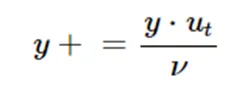
Where y+ = thickness of the first mesh element,

Y = distance from the wall.

U_t = frictional velocity,

nu = dynamic viscosity.

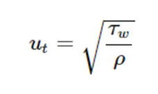
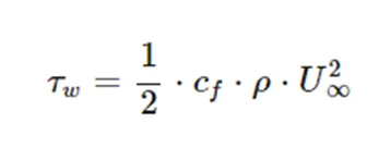
Where = wall shear stress.

C_{f =} skin friction coefficient.

Modelling Approach:

The work flow in Ansys Fluent would follow four steps:

1. Geometry creation.
2. Mesh generation.
3. Pre-processing settings and simulation.
4. Extracting results.

Geometry creation:

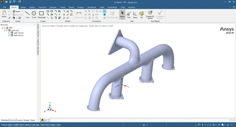
We drag and drop the Fluent module to create the standalone system. We open the geometry editing section- Space claim. We import the given geometry to Space claim and create the fluid volume using Prepare -> Volume Extract -> Select the edges. We crate a new component of the solid volume in the Structure section.

We check for any duplicate or unnecessary edges or faces in the body using Repair -> Split Edges. We use Share option to ensure proper flow of fluid data in the geometry.

Mesh generation:

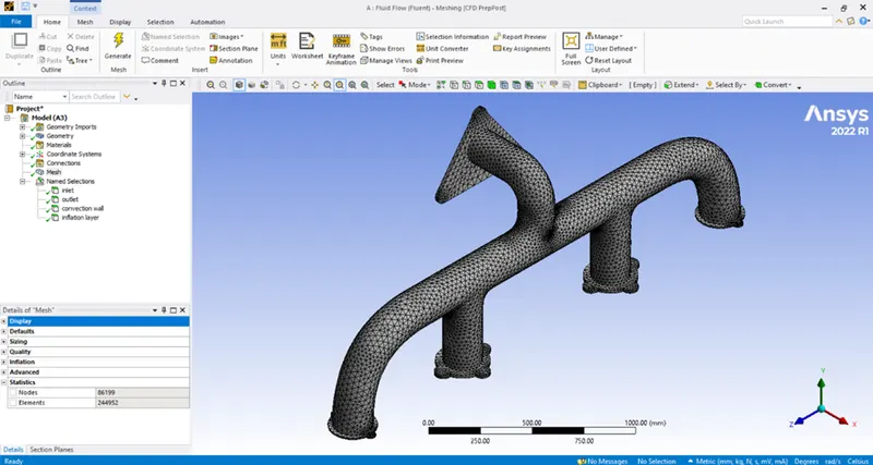
It is a good practice to generate a baseline mesh and perform the simulation to understand the physics and then proceed to the mesh refinement as required. So, we generate the mesh with the default value of mesh length as 0.15m. We can use Inflation, to create a fine structural mesh to capture the flow characteristics along the geometry.

We assign appropriate named selections to make it easier to work in the simulation section later. Here, we assigned the flow inlets, outlet, inflation layer and convection wall. We close the window and the changes are updated in the system.

Using the y+ concept, we calculated first layer thickness as 0.5mm.

Pre-processing settings and Simulation:

We would proceed to Setup the conditions of the model. The process flow would be as follows:

1. Check the mesh in the solver.
2. Choose the turbulence model.
3. Specify boundary conditions.
4. Create necessary surface plots that we need to investigate.
5. We initialize and run the simulation for given number of iterations.

Extracting results:

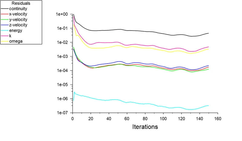
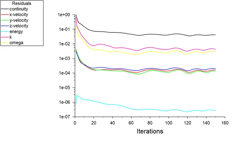
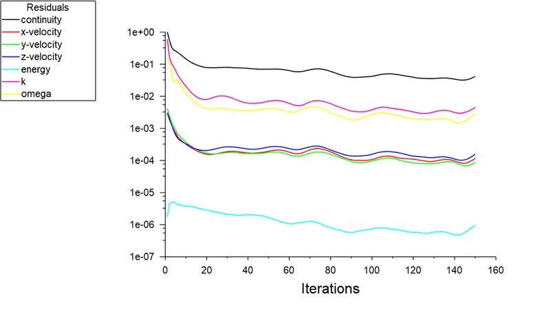
We open the results section where we can use various visualizing tools like transparency and colouring the created surfaces with the instantaneous variables like temperature, velocity and obtain contours, charts and plots. We need to run the simulation until the residual values are either reach the convergence criteria or display a periodic pattern.

Settings used for current simulation:

We used Pressure-based solver, absolute velocity formulation, steady state simulation.

We used k-omega SST turbulence model. We use air as the working media.

We would use fluid velocity as 5 m/s and update the heat transfer coefficient at convectional wall as 20 W/m²K.

Grid Dependency test:

We have to ensure that the solution does not depend on the number of elements in the model. So, we run few simulations with different number of mesh elements. This is called Grid dependency test, where we decide the minimum number of elements required to make sure the solution is acceptable.

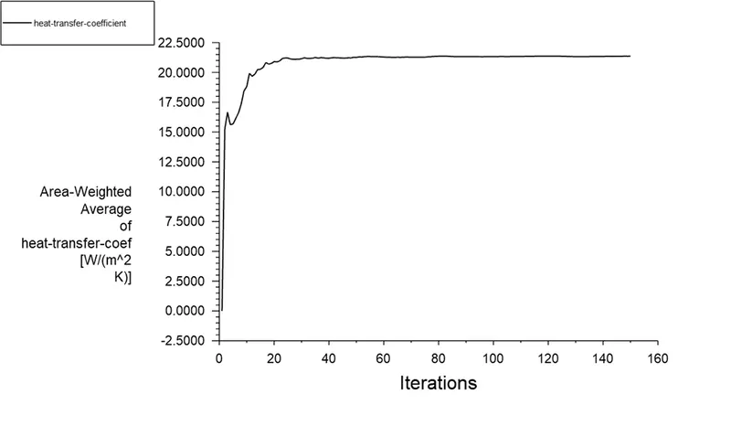
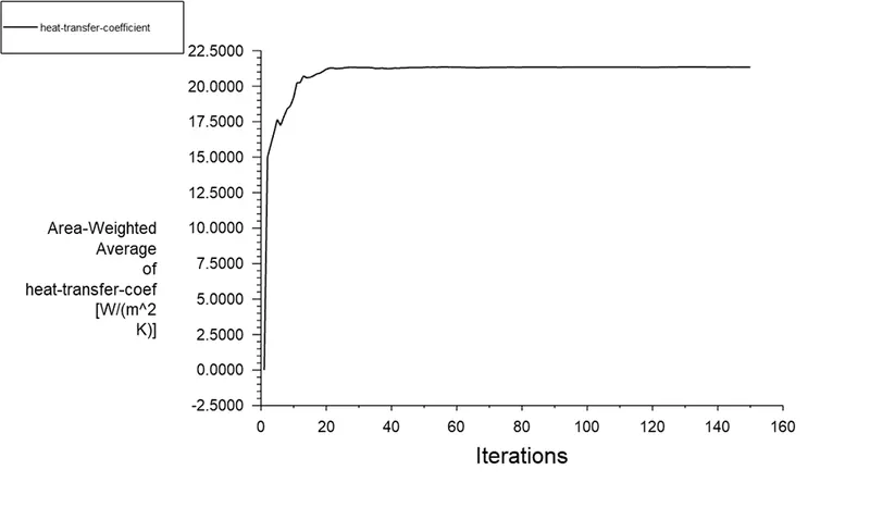
For the given geometry, we would run grid dependency test till we reach a point where we get solutions with acceptable error range (<0.5%). We will use the average value of heat transfer coefficient at inflation layer as the parameter to obtain the ideal computational grid.

Case 1- 150mm:

Scaled residuals:

Average Heat transfer coefficient:

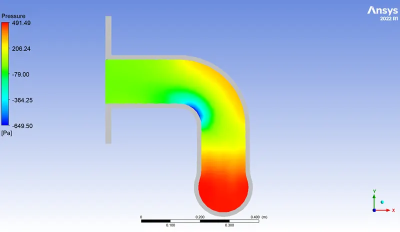
Pressure contour:

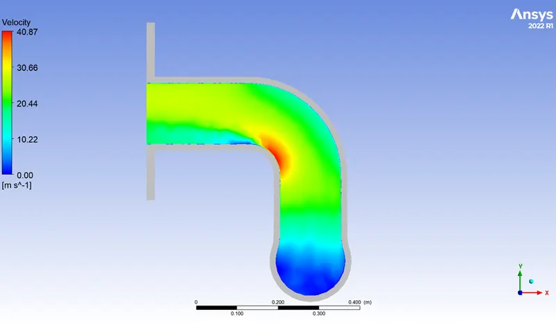
Velocity contour:

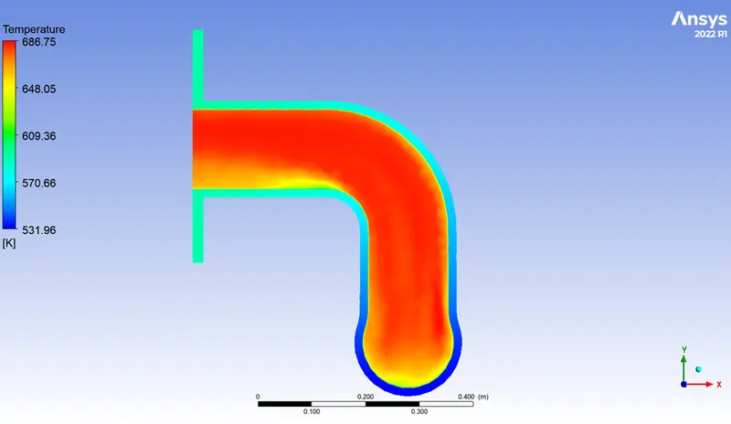
Temperature contour:

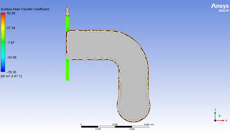
Heat transfer coefficient:

Case 2- 100mm:

Scaled residuals:

Average Heat transfer coefficient:

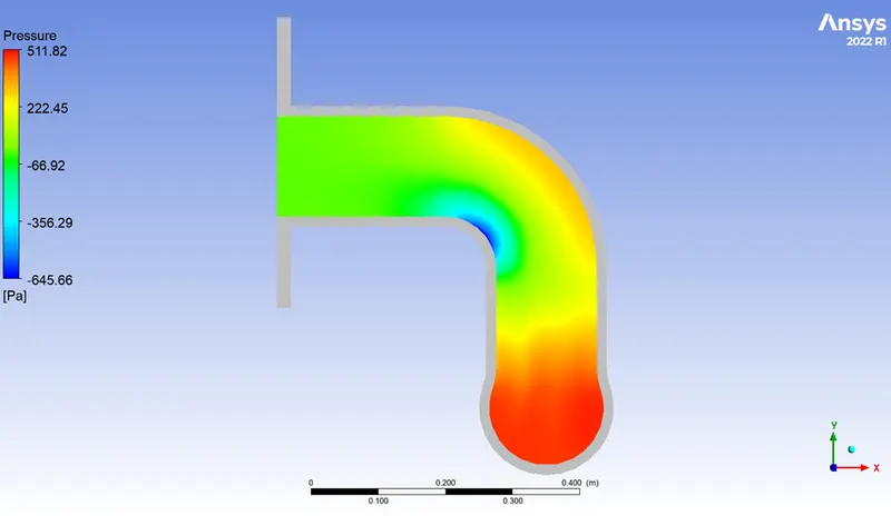
Pressure contour:

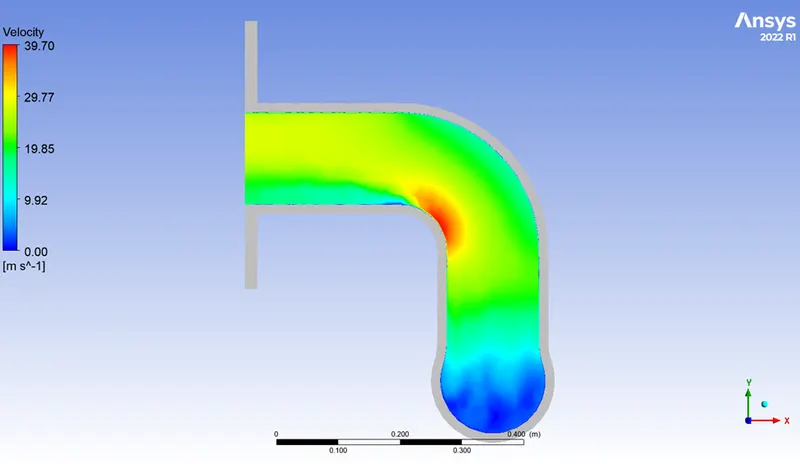
Velocity contour:

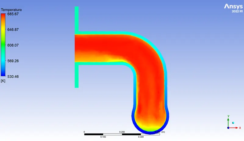
Temperature contour:

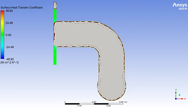
Heat transfer coefficient:

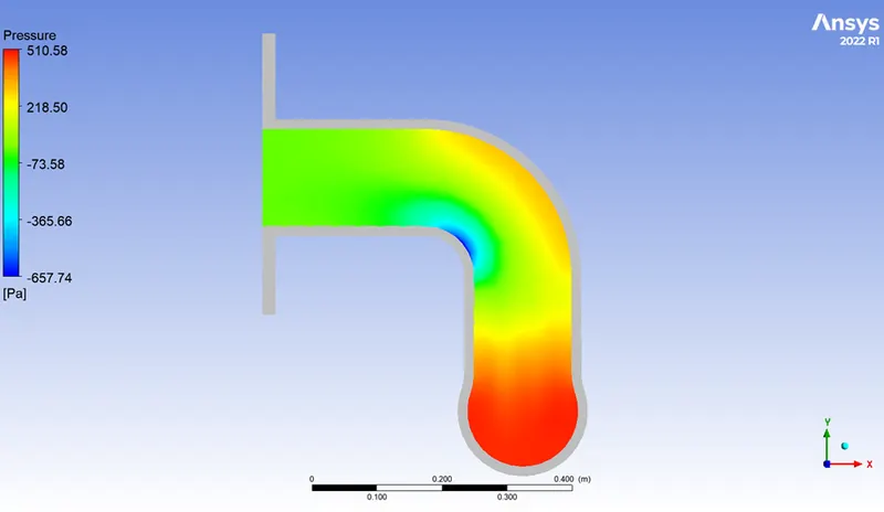
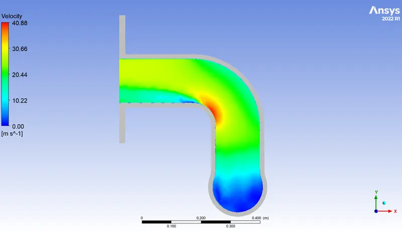
Case 3- 10mm:

Scaled residuals:

Average Heat transfer coefficient:

Pressure contour:

Velocity contour:

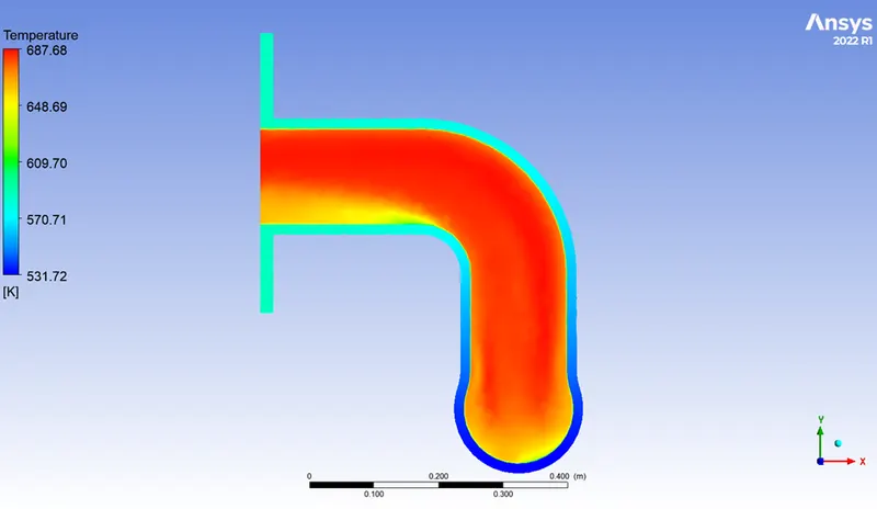
Temperature contour:

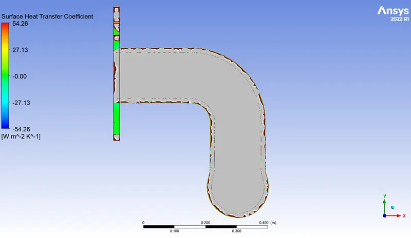
Heat transfer coefficient:

Mesh length(mm)	No. of elements	h (W/m2. K)	Error in h value
150	244952	21.362	-
100	245250	21.349	0.06 %
10	333130	21.337	0.05 %

Since the value of heat transfer coefficient is nearly same for all the computational grids, we can go with the second case with element size 100mm, which has a good visualization of flow parameters in all the property contours.

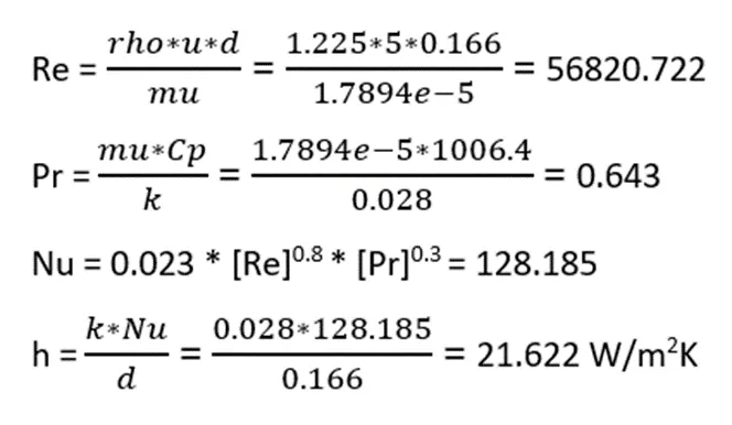
Analytical solution:

The input parameters of the fluid used for the calculation as follows:

Velocity at inlet (u) = 5 m/s

Density of fluid (rho) = 1.225 kg/m³

Characteristic length (d) = 0.166 m

Dynamic viscosity of fluid (mu) = 1.7894e-5 Ns/m²

Thermal conductivity (k) = 0.028 W/mK

Specific heat (C_P) = 1006.4 J/kgK

Validation of Results:

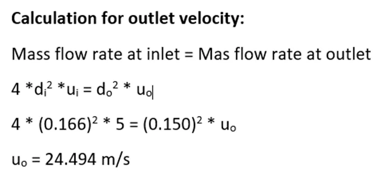
The analytical value obtained for the given problem is 21.622 whereas the computational solution obtained is 21.349 W/m². K. The deviation in the value is 1.26%. Since the deviation is less than 5%, we can say the turbulence model with the given computational grid managed to capture the physics of the flow very accurately. We get the outlet velocity at outlet as 25.276 m/s. The deviation is 3.19% which is within acceptable range. Hence, the numerical solution obtained is valid.

Conclusion:

The errors in the experimental and simulated values are very small. Hence, we can say the turbulence model and the computational grid captured the flow physics accurately.

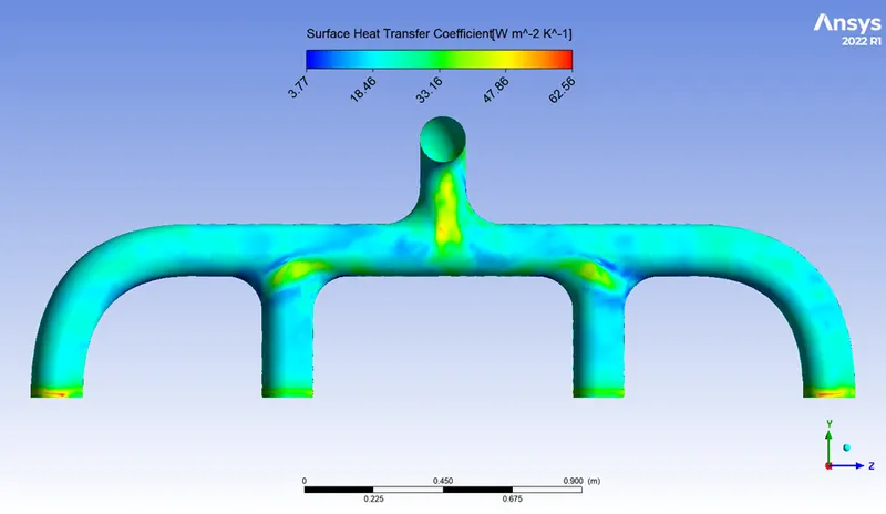
It is also observed at that at the bend in the pipe the velocity magnitude is maximum. This can be because of the sudden addition of the velocity components in other two co-ordinate axis. Since the velocity increases at the bends, the mass flow rate at the bend region increases, thus heat transfer coefficient at these regions also increases as shown by the yellow regions of the following contour.

References:

1. https://www.cadence.com/ko_KR/home/tools/system-analysis/computational-fluid-dynamics/y-plus.html - Tool used to compute y+ value.
2. Zhang, Li-Zhi, Conjugate Heat and Mass Transfer in Heat Mass Exchanger Ducts, Academic Press Inc., 2013.