Week 4 - CHT Analysis on Exhaust port

Aim: To simulate flow through the exhaust manifold wherein 4 inlet port is connected to 1 outlet port. Velocity, Pressure, heat transfer coefficient and Nusselt number for the flow are simulated for the manifold.

Conjugate Heat Transfer:

• In real world the heat transfer takes from solid and fluid, in solids conduction dominates and in fluids convection dominates. Conjugate heat transfer is used to solve the heat transfer between solid and fluid wherein energy is transferred between the interface of two body.
• This method is very much useful in optimizing the design of the product and construct the design such that the energy efficiency is maximised at low cost.
• Conjugate heat transfer method is used to design the Heat exchanger, HVAC equipment, electronic equipment, Engine cooling system and various general-purpose equipment etc.

Analytical Solution:

For Air,

Density =1.225, Viscosity= 1.7894e-5 Kg/ms, Thermal conductivity= 0.0242W/mK, Specific heat capacity= 1006.43j/KgK

For Aluminium,

Density= 2719Kg/m^3, Specific heat capacity= 871J/KgK, Thermal conductivity= 202.4W/mK

According to the Sieder Tate relation which correlates the Nu number with Re and Pr

`Nu=0.027*Re^0.8*Pr^n`

where, n= 0.3 for fluid being cooled

n= 0.4 for fluid being heated

Reynolds Number (Re): `= (rho*V*L)/(mu)=(1.225*5*0.166)/(1.7894*10^(-5) ) =56,820.722`

Prandlt Number (Pr): `=(mu*Cp)/K=(1.7894*10^(-5)*1006.43)/0.0242=0.744`

Nusselt Number(Nu): `=0.023*(56820.722)^0.8*(0.744)^0.3=133.907`

Also, `Nu=(h*L)/K`

so, Convective Heat Transfer Coefficient (h): `=(Nu*K)/L=(133.907*0.0242)/0.166=19.521w/(m^2*K)`

Baseline Simulation:

It is used to estimate the overall simulation using coarse mesh and helps us to identify the refinement required for the finer mesh solution.

Steps for Baseline Simulation:

• Manifold part is imported within the Ansys geometry, then the extra edges are removed using Repair extra edges and select manually the extra edges and select ok or one could directly select ok in the window which automatically removes the extra edges from complex geometry.
• The volume from the exhaust manifold is extracted and named fluid volume in the thread. Then from the geometry thread select the solid and name it solid volume.
• Now select Solid and Fluid volume from the thread and right click and select move to new component and then delete the above parts as it has no data within it.
• From the Workbench select the share topology or else while meshing the geometry Ansys will mesh it as two separate components.

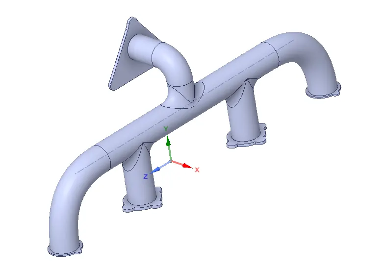
• Select the different component and name them using N.
• Generate coarse mesh for the component with element size of 0.15m
• Make sure that the element quality is above 10%

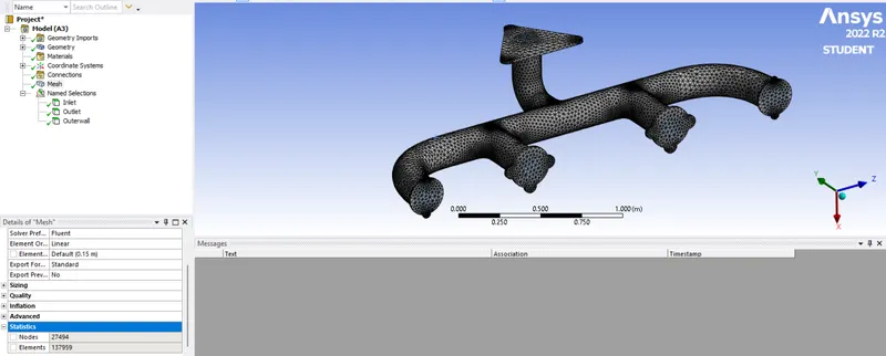
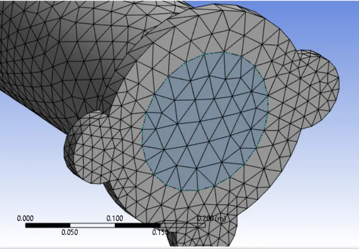
• From the setup select K-epsilon, standard wall function turbulence model. Steady state, Pressure based and absolute method.
• From the material select fluid as air and solid as aluminium. The boundary condition for Inlet as 5m/s velocity, 700K temperature. For Outlet gauge pressure = 0, For Outer wall select convective and heat transfer coefficient= 20W/m^2*K. Flange and other component select the heat flux and zero value i.e. adiabatic condition. And other parts as wall boundary condition.
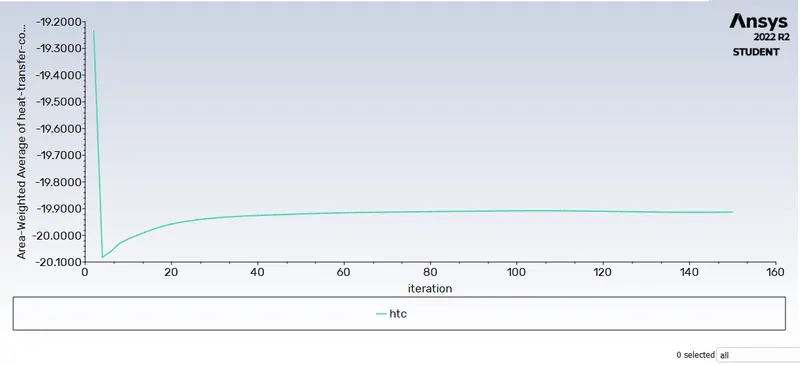
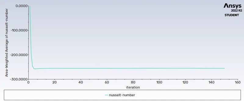
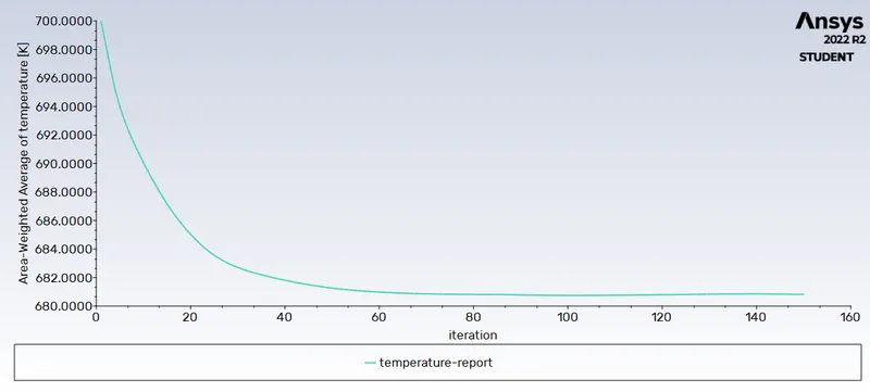
• Generate the report for the Weighted average for the outlet temperature, surface Nusselt number and Surface Heat transfer coefficient.
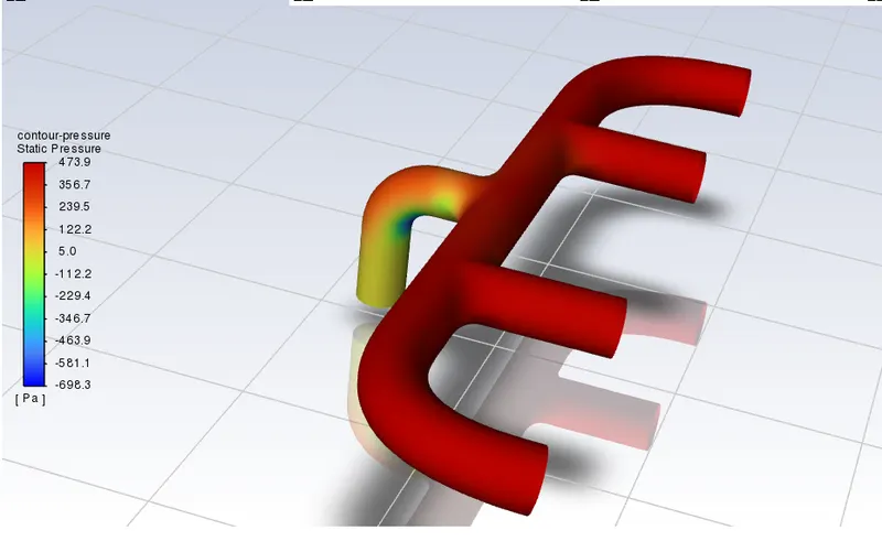
• Create the contour for Pressure, temperature, streamline and others etc.
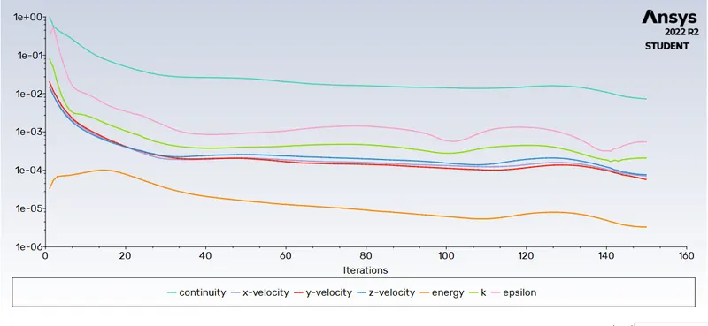
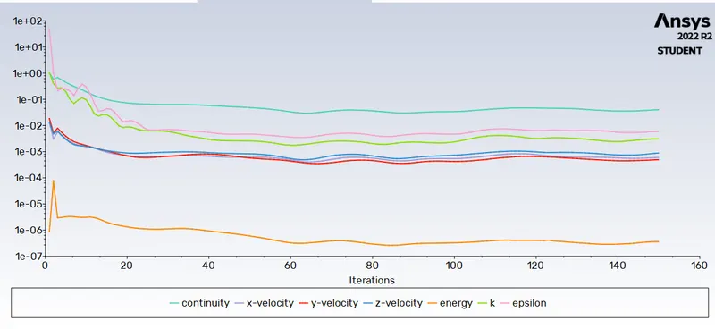
• Initialise the problem and solve for 150 iteration.

Residual Plot:

Surface Wall Heat Transfer Coefficient Plot:

Surface Nusselt Number Plot:

Area Weighted Outlet Temperature Plot:

Pressure Contour:

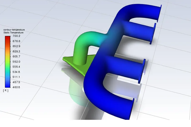
Temperature Contour:

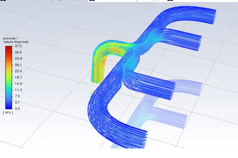
Streamline:

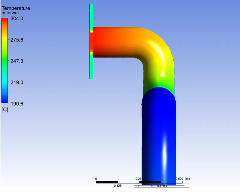
Outer Wall Temperature Contour:

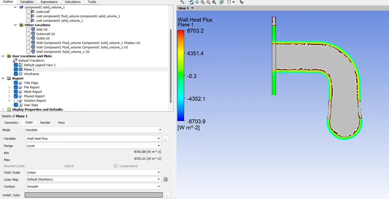
Outlet Plane Heat Flux Contour:

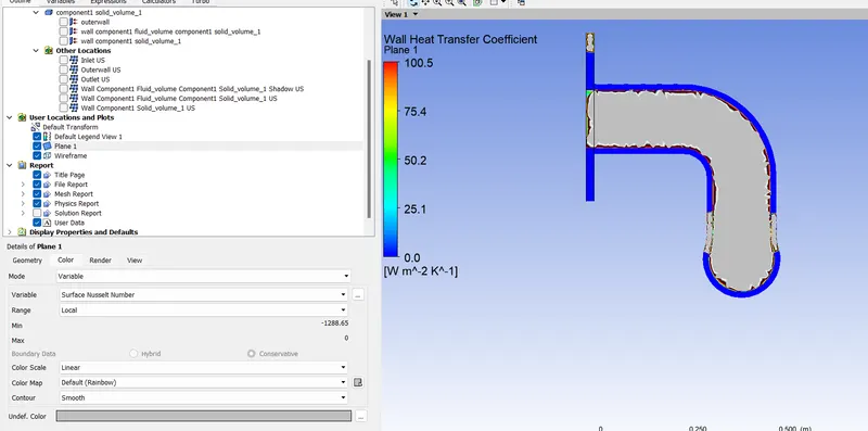
Outlet Plane Heat Transfer Cofficient:

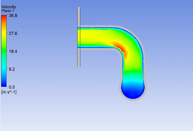
Outlet Plane Velocity Contour:

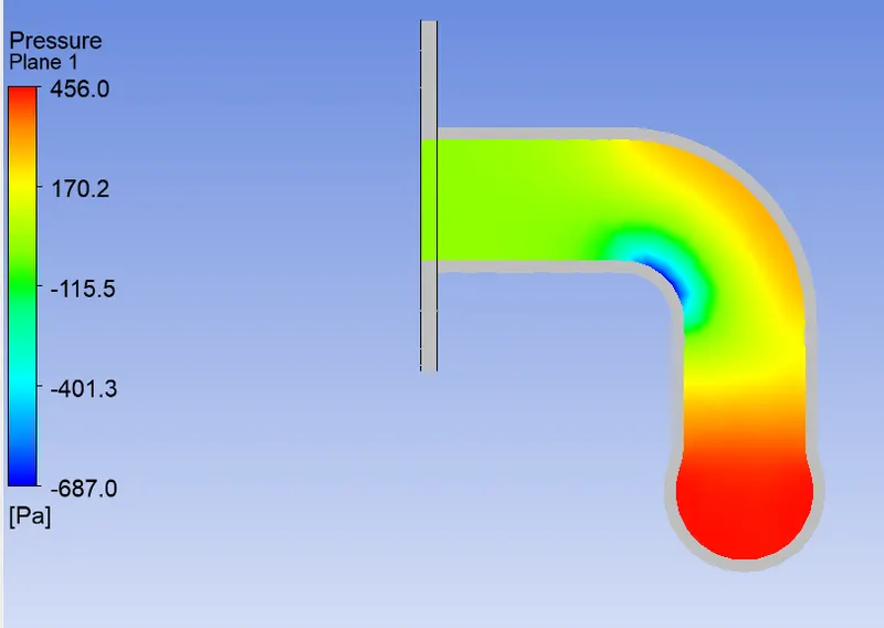
Outlet Plane Pressure Contour:

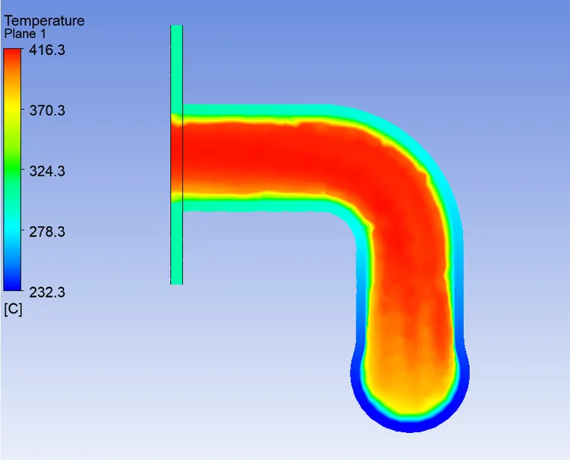
Outlet Plane Temperature Contour:

Result_1:

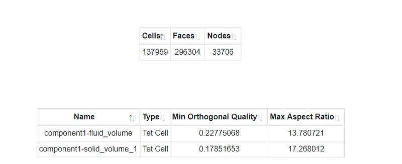
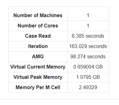
Finer Mesh Simulation:

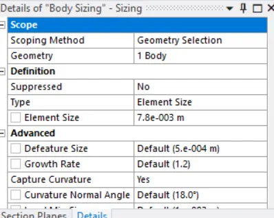
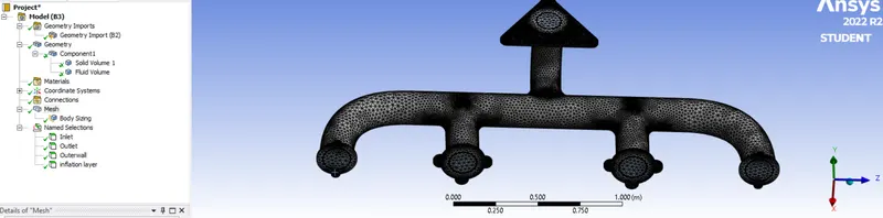
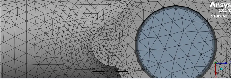
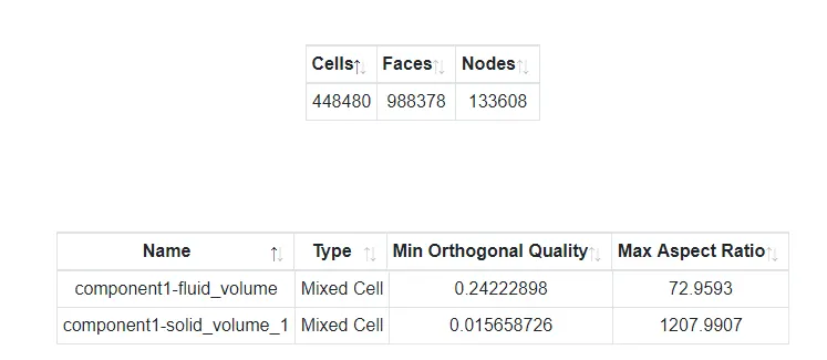
• We try to find the heat transfer coefficient which could be found from the fluid cell adjacent to the solid wall, in order to find the thickness of the cell according to Y+ method for 30 to 300 as going below that will lead to mesh cell more than 0.5 million which is difficult to solve in trial version of Ansys.
• We generate the mesh as per the figure.

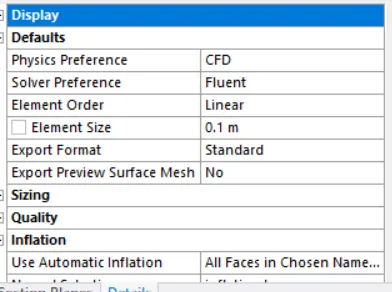
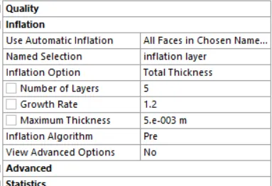
• All other settings are now similar to the coarse mesh simulation.

Residual Plot:

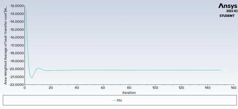
Surface Wall Heat Transfer Coefficient Plot:

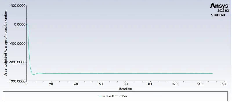
Surface Nusselt Number Plot:

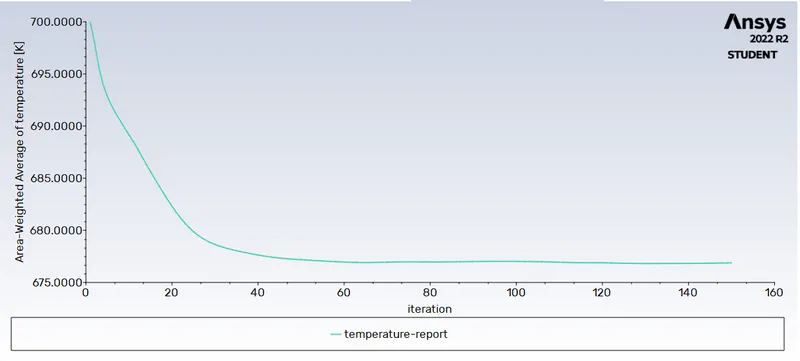
Area Weighted Outlet Temperature Plot:

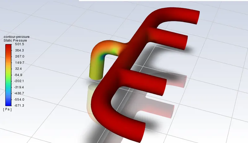
Pressure Contour:

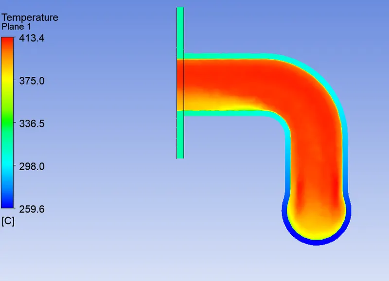
Temperature Contour:

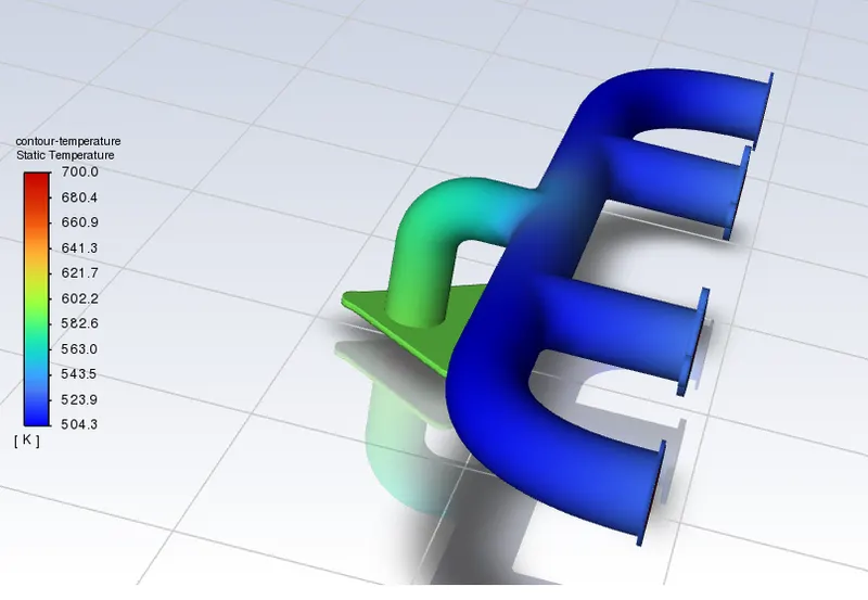
Streamline:

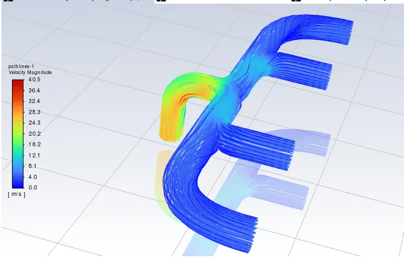
Outer Wall Temperature Contour:

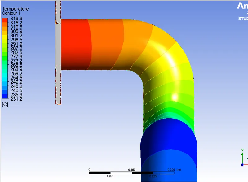
Outlet Plane Heat Flux Contour:

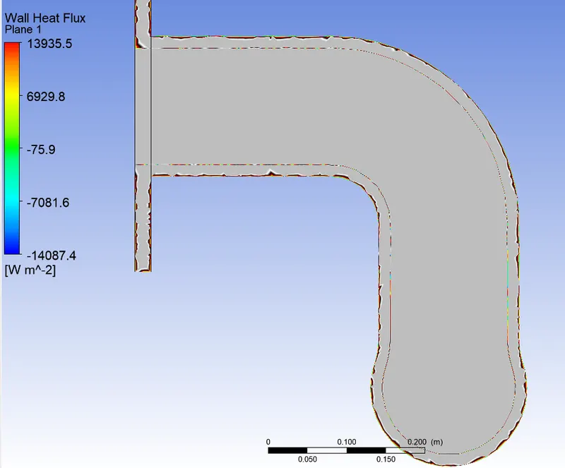
Outlet Plane Heat Transfer Cofficient:

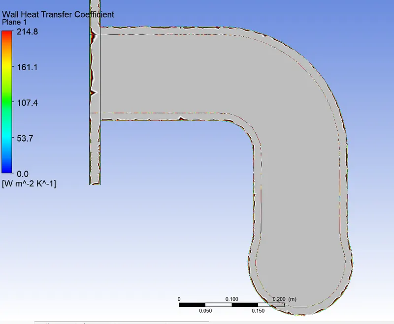
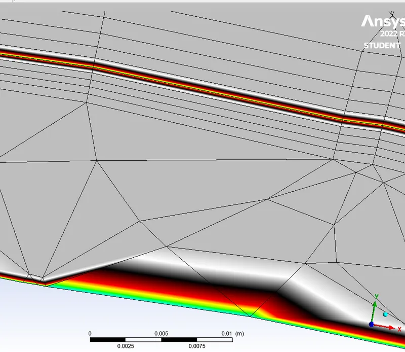
• Heat Transfer Coefficent value is calculated from the first cell in contact with fluid and solid

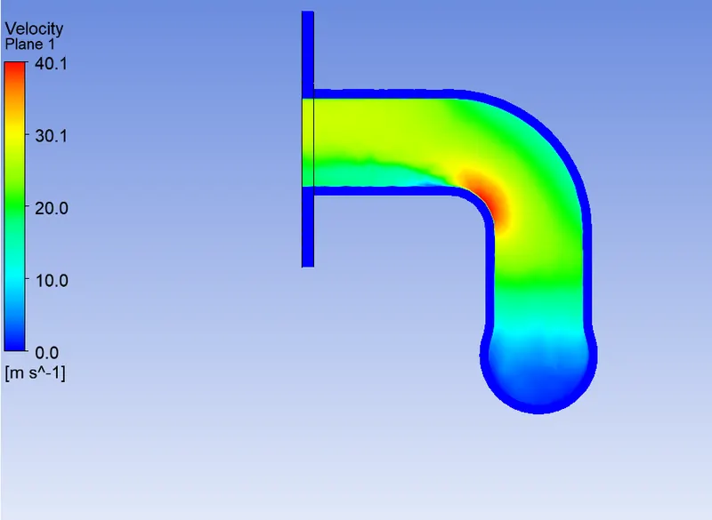
Outlet Plane Velocity Contour:

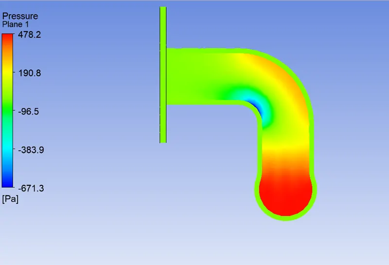
Outlet Plane Pressure Contour:

Outlet Plane Temperature Contour:

Result_2:

Validation:

Parameters	Coarse Mesh	Fine Mesh	Analytical Result
No. of Element	1,37,959	4,48,480	-
Outlet Temperature (*K)	680.82	676.89	-
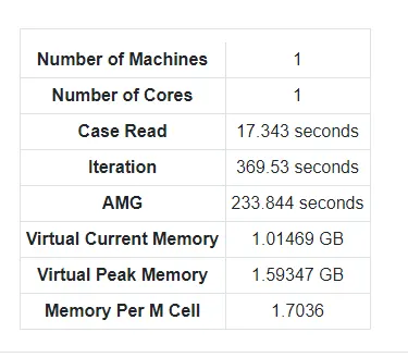
Time in Second	163.09	369.53	-
Surface wall Heat Transfer Coefficient	19.912	20.159	19.521
% Error for HTC	2.003	3.268	0
Surface Nusselt Number	255.119	258.667	133.907
Max. Wall temperature (*C)	304	319.9	-

Conclusion:

• The effect of element size can be seen in the above result.
• Results get converged towards the actual as the no. of elements gets increased.
• Results of the simulation is not much affected by the no. of element size.

Accuracy of the HTC depends upon:

• The no. of element and element size of Mesh.
• According to the selection of Y+ value for Inflation layer thickness.
• Selection of fluid & solid material and their properties.
• Defining proper boundary condition for the simulation.
• Selection of proper Turbulence model for the simulation.