Week 4 - CHT Analysis on Exhaust port

CHT ANALAYSIS ON AN EXHAUST PORT

The following project deals with the CHT analysis of an exhaust port of an inline-4-cylinder engine.

CHT ANALYSIS

Conjugate heat transfer (CHT) analysis can accurately predict heat transfer by simultaneous solving all the relevant solid and flow field heat transfer processes, for example: conduction through solids, free and forced convection in the gases/fluids and thermal radiation.

Typical applications of this analysis type exist as, but are not limited to, the simulation of heat exchangers, cooling of electronic equipment, and general-purpose cooling and heating systems.

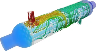
Natural convection around a heat exchanger. Cold water enters in and gets heated due to hot air flowing opposite to it.

One simple way to realize conjugation is to apply the iterations. The idea of this approach is that each solution for the body or for the fluid produces a boundary condition for other components of the system. The process starts by assuming that one of conjugate conditions exists on the interface. Then, one solves the problem for body or for fluid applying the guessing boundary condition and uses the result as a boundary condition for solving a set of equations for another component, and so on. If this process converges, the desired accuracy may be achieved. However, the rate of convergence highly depends on the first guessing condition, and there is no way to find a proper one, except through trial and error.

Another numerical conjugate procedure is grounded on the simultaneous solution of a large set of governing equations for both subdomains and conjugate conditions. Patankar proposed a method and software for such solutions using one generalized expression for continuously computing the velocities and temperature fields through the whole problem domain while satisfying the conjugate boundary conditions.

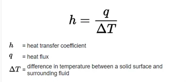
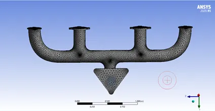
The problem will be approached by first creating a baseline mesh and then refining it further to get more accurate results.

Boundary Conditions

Inlet	Velocity=5ms^-1, Temperature=700k
Outer Wall	Heat Transfer Coefficient=20w/m^2-k

The equations solved are RANS and Energy equation. The Turbulence model selected is k-ε turbulence model.

GEOMETRY

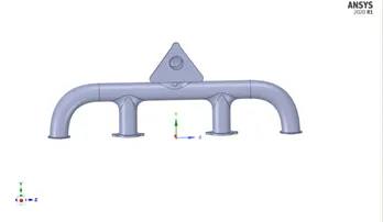
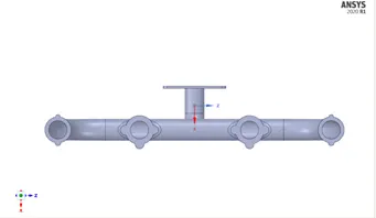
Case 1(Baseline Mesh)

Results

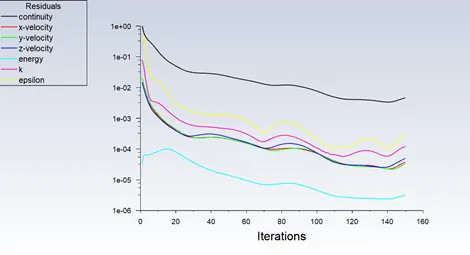
Residuals
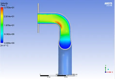
Velocity Contour
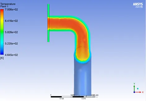
Temperature Contour
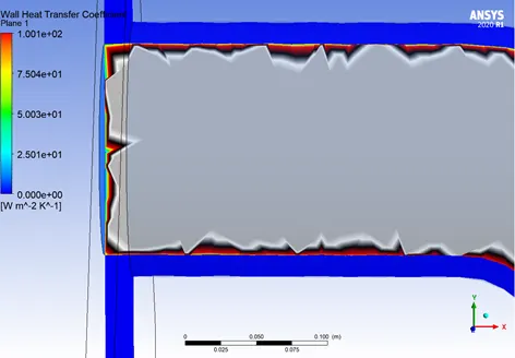
Heat Transfer Coefficient

Heat Transfer Coefficient

108.7 W/(m2•K)

CASE 2 (REFINED MESH)

Results

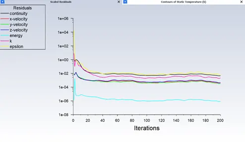
Residuals
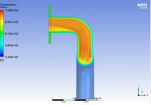
Temperature Contour
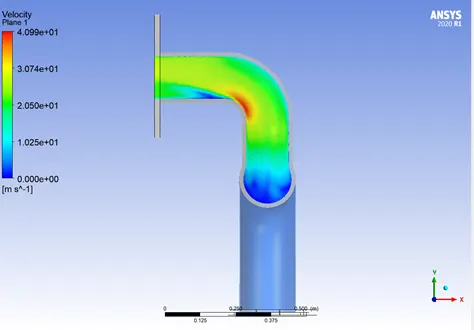
Velocity Contour

Heat Transfer Coefficient

221.85678 W/(m2•K)

Observations

It is observed that temperature in the outlet region is very high despite the inlets having hotter air pumped in. This can be explained by taking into the account that the outlet velocity is high which results in higher Reynolds number in that region. This results in high Heat Transfer Coefficient which explains the high temperature in the outlet.

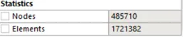
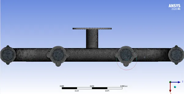
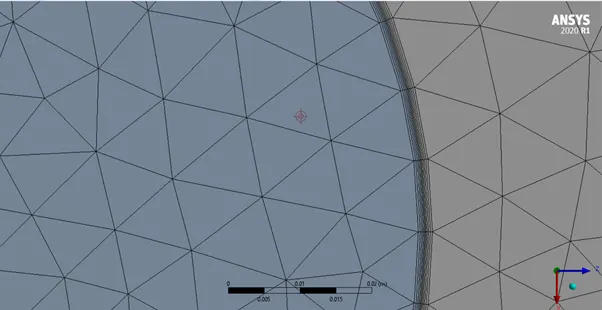
The velocity and temperature plots of Case 2 is observed to be smoother. This is because in Case 2 the mesh has been refined. We have added Inflation layers and Body sizing to get accurate results. The value of HTC in case 2 is more accurate due to this.

Verification

The results obtained in this simulation are like those done experimentally (from genuine sources). Hence, the results can be verified.

Some of the steps to obtain better results

Using Hexagonal elements

When determining whether to use hexahedral (hex) elements or tetrahedral elements in an FEA model configuration, it’s important to keep in mind the overall shape and complexity of the object itself. The general rule of thumb is to mesh with hexahedral elements if possible. Hex or “brick” elements generally result in more accurate results at lower element counts than tetrahedral elements. However, if the object contains acute angles or other complex geometries, it may be necessary to mesh with tetrahedral elements.

Mesh Size and Order

Properly understanding mesh order and size are key to finding the balance between accurate results and reasonable run times in a finite element analysis. Mesh size simply refers to the characteristic edge length of an element. A smaller mesh size will result in more elements in the model, resulting in longer run times and more accurate results. Order describes the shape function used to calculate element displacements. First-order elements have nodes only at the corners of the elements and calculate displacement linearly between nodes. Second-order elements include midsize nodes between the corners and calculate displacement quadratically. The additional detail in second-order elements typically results in increased accuracy, but at a significantly increased computational cost.

Running the simulations until it converges

Regarding the convergence criterion, residuals history hands over meaningful insights over convergence. Generally, residuals decrease, and stabilization are good signs of proper solution convergence. Nevertheless, these alone should not be considered as strict convergence criterion.

Regarding the convergence criterion, residuals history hands over meaningful insights over convergence. Generally, residuals decrease and stabilization are good signs of proper solution convergence. Nevertheless, these alone should not be considered as strict convergence criterion.