Ahmed Body Challenge

STUDY OF FLOW OVER AHMED BODY

The following study involves conducting flow simulations over an Ahmed Body and making various conclusions from it.

Objectives of the Study

• Describing Ahmed Body and its importance
• Explaining the reason for the negative pressure in wake region
• Explaining the significance of point of separation

Ahmed Body

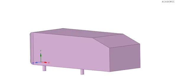
The Ahmed body is a generic car body (a simplified vehicle model). The airflow around the Ahmed body captures the essential flow features around an automobile and was first defined and characterized in the experimental work of Ahmed. Although it has a very simple shape, Ahmed body allows us to capture characteristic features that are relevant to bodies in the automobile industry.

This model is also used to describe the turbulent flow field around a car-like geometry. Once the numerical model in validated, it is used to design new models of the car.

GEOMETRY

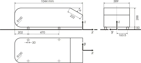
HEIGHT	288mm
WIDTH	389mm
LENGTH	1044mm
SLANT	40°

What is its importance?

This model is used to describe the turbulent flow field around a car-like geometry. Once the numerical model in validated, it is used to design new models of the car.

In todays scenario, cars are complex in shape hence are challenging to design and difficult to compute aerodynamic drag, so Ahmed Body has become a benchmark for aerodynamic simulation tool.

Vehicle manufacturers compete to increase vehicle efficiency by improving size, shape, weight and drag. To decrease drag, companies try to lower drag efficiency of the body by improving the shape. The lower the drag coefficient the more the vehicle efficiency which results in more speed and fuel efficiency.

Solving and Modelling Approach

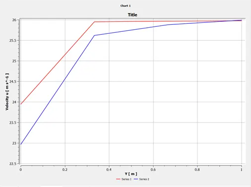
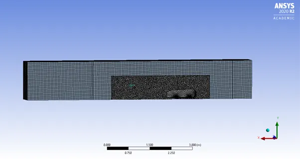
The grid independence test is done by using two enclosures around the Ahmed Body. Hexagonal meshes are used because it gives more refinement and more accurate results.

The turbulence model used is k-epsilon and Standard wall functions are used. The modelling is done on pressure-based solver.

An interference check is done to maintain uniformity throughout the mesh and the two different meshes don’t interfere.

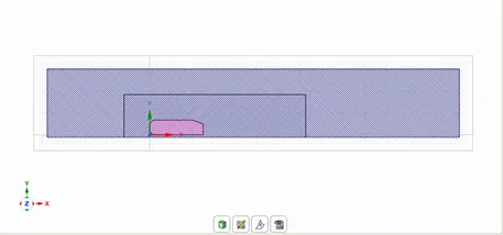
Enclosure and Boundary Conditions

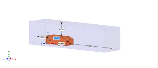
Smaller enclosure

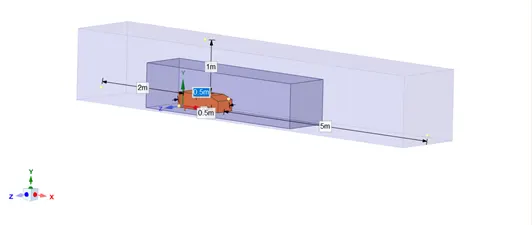
Larger Enclosure

Boundary conditions

Inlet velocity	25 m/s
Outlet pressure	0 atm
Inlet temperature	300 K
Material used	Air
Density of material	1.225 kg/m^3
Viscosity of material	1.81x10^-5 kg/ms

The modelling is done in 3 cases, in each case the mesh is refined further.

Case 1(222359 elements)

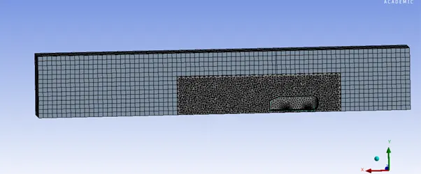
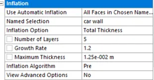
The following setup is used

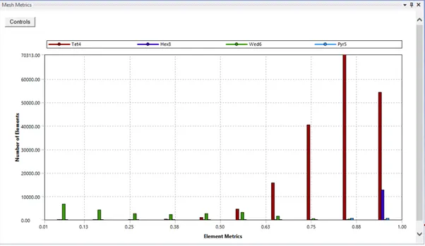
Clearly the Mesh quality is excellent. Most elements have quality between 75-100% and very few elements have quality less than 60%.

Results

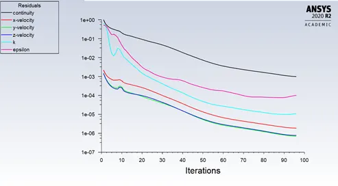
Residuals
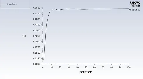
Lift Coefficient
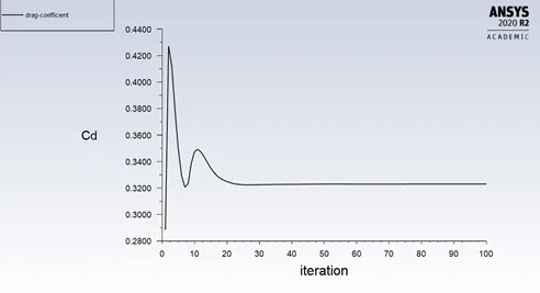
Drag Coefficient
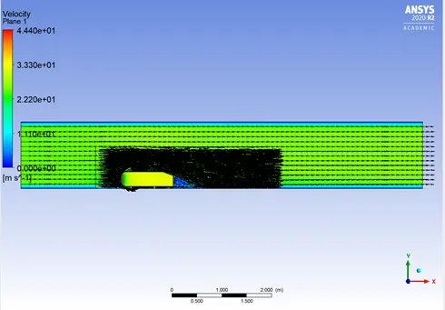
Vector Plot
Velocity Contour
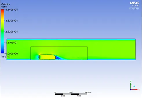Chart of line velocity

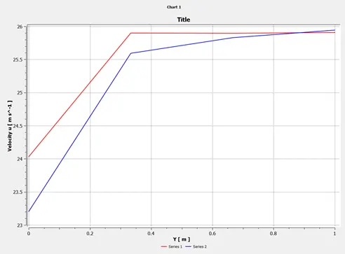Lift Coefficient	0.245
Drag Coefficient	0.323

Case 2(285819 elements)

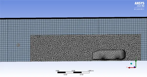
The setup used is same as that of Case 1

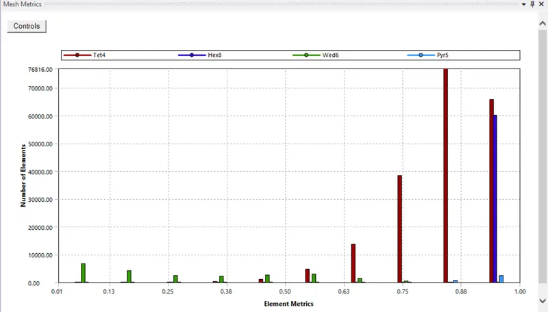
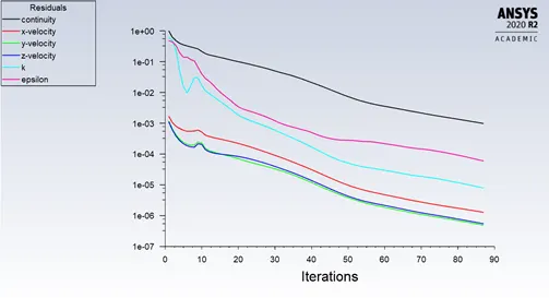
Clearly the Mesh quality is excellent. Most elements have quality between 75-100% and very few elements have quality less than 60%.

Results

Residuals
Lift Coefficient
Drag Coefficient
Vector Plot
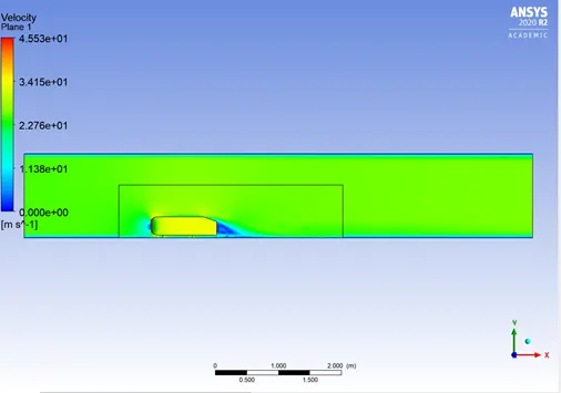
Velocity Contour
Chart of line velocity

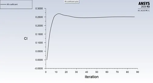
Lift Coefficient	0.2503
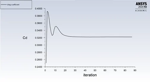
Drag Coefficient	0.3219

Case 3(339203 elements)

The setup used is same as that of case 1

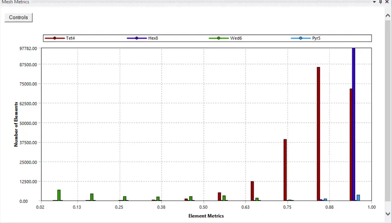
Clearly the Mesh quality is excellent. Most elements have quality between 75-100% and very few elements have quality less than 60%.

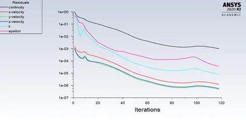
Results

Residuals
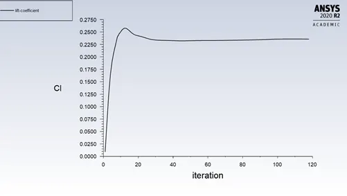
Lift Coefficient
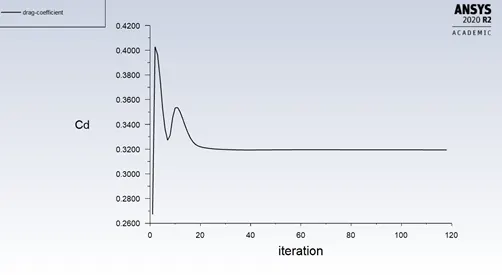
Drag Coefficient
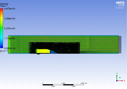
Vector Plot
Velocity Contour
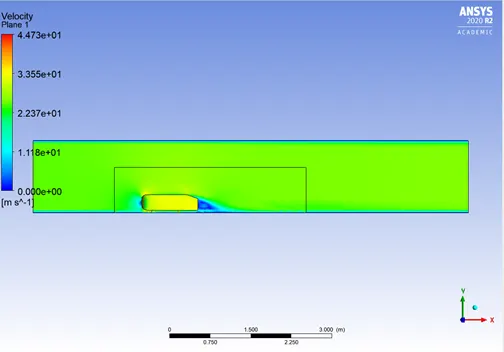Chart of line velocity

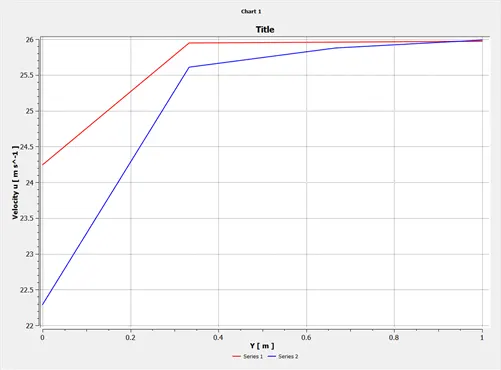Lift Coefficient	0.253
Drag Coefficient	0.319

Observations and Conclusions

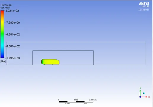
It is observed that there is negative pressure in the wake region.

Why is this?

Pressure gradient is an is one of the factors that influences a flow immensely. It is easy to see that the shear stress caused by viscosity has a retarding effect upon the flow. This effect can however be overcome if there is a negative pressure gradient offered to the flow. A negative pressure gradient is termed a Favourable pressure gradient. Such a gradient enables the flow. A positive pressure gradient has the opposite effect and is termed the Adverse Pressure Gradient. Fluid might find it difficult to negotiate an adverse pressure gradient. Sometimes, we say the the fluid must climb the pressure hill.

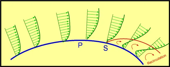
One of the severe effects of an adverse pressure gradient is to separate the flow. Consider flow past a curved surface as shown in Fig.6.4. The geometry of the surface is such that we have a favourable gradient in pressure to start with and up to a point P. The negative pressure gradient will counteract the retarding effect of the shear stress (which is due to viscosity) in the boundary layer. For the geometry considered we have a an adverse pressure gradient downstream of P.

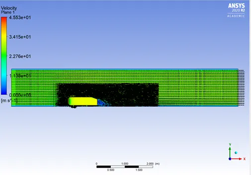
Now the adverse pressure gradient begins to retard. This effect is felt more strongly in the regions close to the wall where the momentum is lower than in the regions near the free stream. As indicated in the figure, the velocity near the wall reduces and the boundary layer thickens. A continuous retardation of flow brings the wall shear stress at the point S on the wall to zero. From this point onwards the shear stress becomes negative and the flow reverses and a region of recirculating flow develops. We see that the flow no longer follows the contour of the body. We say that the flow has separated. The point S where the shear stress is zero is called the Point of Separation.

Depending on the flow conditions the recirculating flow terminate and the flow may become reattached to the body. A separation bubble is formed. There are a variety of factors that could influence this reattachment. The pressure gradient may be now favourable due to body geometry and other reasons. The other factor is that the flow initially laminar may undergo transition within the bubble and may become turbulent. A turbulent flow has more energy and momentum than a laminar flow. This can kill separation and the flow may reattach. A short bubble may not be of much consequence.

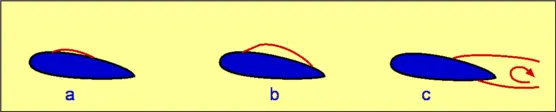
On aerofoils sometimes the separation occurs near the leading edge and gives rise to a short bubble. What can be dangerous is the separation occurring more towards the trailing edge and the flow not reattaching. In this situation the separated region merges with the wake and may result in stall of the aerofoil (loss of lift).

Conclusion

Although the data has quantitative differences, it is qualitatively accurate because the values of the drag coefficients are so close. This simulation is more than accurate enough to calculate drag coefficients