Week 5 - Rayleigh Taylor Instability
RAYLEIGH TAYLOR INSTABILITY CHALLENGE
The following is a study based on developing CFD models to solve Rayleigh Taylor instability problems and calculating the Atwood Number for different cases for multiphase flows.
THEORY
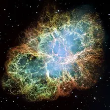
The Rayleigh–Taylor instability, or RT instability is an instability of an interface between two fluids of different densities which occurs when the lighter fluid is pushing the heavier fluid. Examples include the behaviour of water suspended above oil in the gravity of Earth, mushroom clouds like those from volcanic eruptions and atmospheric nuclear explosions, supernova explosions in which expanding core gas is accelerated into denser shell gas, instabilities in plasma fusion reactors and inertial confinement fusion.
Water suspended atop oil is an everyday example of Rayleigh–Taylor instability, and it may be modelled by two completely plane-parallel layers of immiscible fluid, the denser on top of the less dense one and both subject to the Earth's gravity. The equilibrium here is unstable to any perturbations or disturbances of the interface: if a parcel of heavier fluid is displaced downward with an equal volume of lighter fluid displaced upwards, the potential energy of the configuration is lower than the initial state.
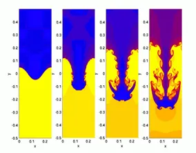
CFD models based on Mathematical analysis of RT instabillity
VOLUME OF FLUID METHOD(VOF)
The VOF method is computationally friendly, as it introduces only one additional equation and thus requires minimal storage. The method is also characterized by its capability of dealing with highly non-linear problems in which the free-surface experiences sharp topological changes. By using the VOF method, one also evades the use of complicated mesh deformation algorithms used by surface-tracking methods. The major difficulty associated with the method is the smearing of the free-surface. This problem originates from excessive diffusion of the transport equation.
k-L Turbulence Model
The k-L turbulence model, where k is the turbulent kinetic energy and L represents the turbulent eddy scale length, is a two-equation turbulence model that has been proposed to simulate turbulence induced by Rayleigh-Taylor and Richtmyer Meshkov instabilities. The model describes the dominant eddies in the mixing zone with evolutionary equations for their characteristic dimension (L) and energy per unit mass (K) .
Kelvin-Helmholtz Instabillity Model
The theory predicts the onset of instability and transition to turbulent flow within fluids of different densities moving at various speeds. It was recently discovered that the fluid equations governing the linear dynamics of the system admit a parity-time symmetry, and the Kelvin–Helmholtz instability occurs when and only when the parity-time symmetry breaks spontaneously
CFD ANALYSIS
A transient pressure based simulation is done. Multipahse(implicit) model is choosen. The flow is assumed to be laminar. Air is taken as the primary phase. Water is taken as secondary phase for Cases 1,2 and 3. A user defined material is taken as secondary pashe for Case 4. Volume of Fluid(VOF) method is selected in this analysis.
A baseline mesh is further refined and analysis are done on each case.
GEOMETRY
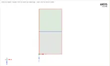
A rectangular geometry is created with 20x20 dimension(top and bottom). The pull tool is used to create surfaces. Share topology is turned on.
CASE 1
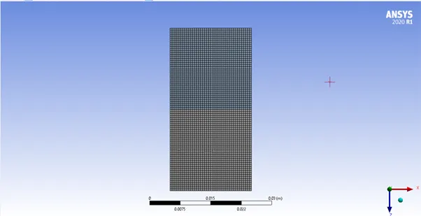
Basic quad mesh is created. Baseline mesh size=0.50mm.
|
NODES |
3321 |
|
ELEMENTS |
3200 |
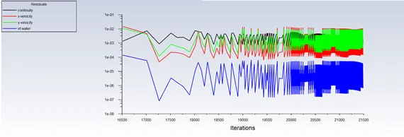
RESULTS
CASE 2
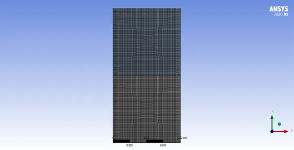
The baseline mesh is further refined. Mesh size=0.25mm.
|
NODES |
13366 |
|
ELEMENTS |
13122 |
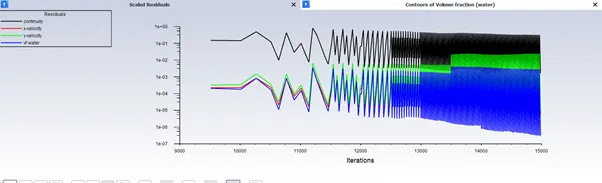
RESULTS
Case 3
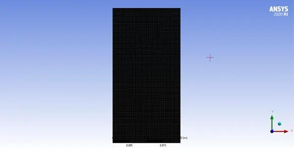
Refined case 2. Mesh size=0.10mm.
|
NODES |
82012 |
|
ELEMENTS |
81406 |
RESULTS
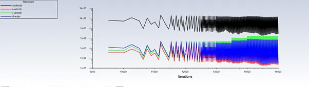
Case 4
Mesh size is same as Case 3. The material used here is a user-defined material with density=400 kg/m^3 and viscosity=0.001 kg/ms^-1 and water.
|
NODES |
82012 |
|
ELEMENTS |
81406 |
RESULTS
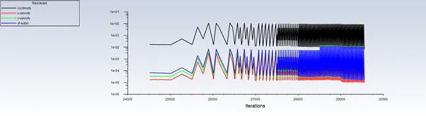
Observations
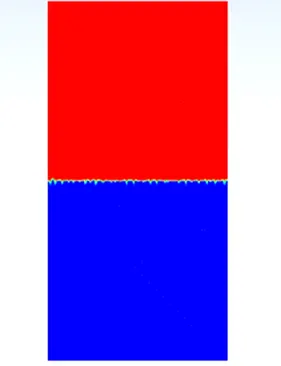
Small pertubrations are generated at the interface. These are similar to Sine waves.
Step 2
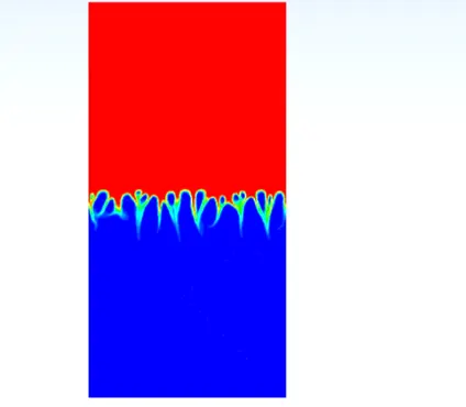
At interface low density bubbles push into higher density liquid. Spikes are also observed. This is a result of high density liquid pushing low density liquid.
Step 3
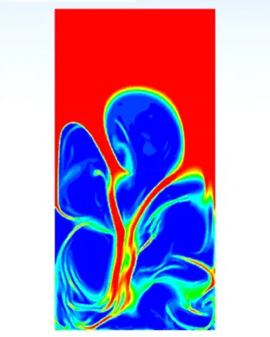
Bubbles and spikes interact with each other to form mushrrom like structures are formed.
Stage 4
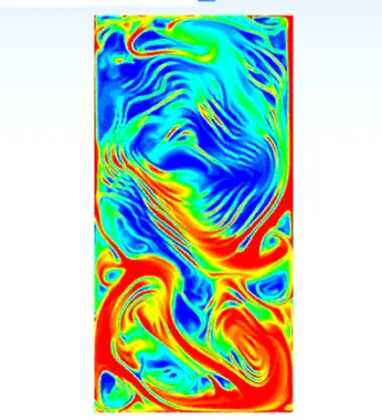
Mixing of fluids happen and instabillity happens due to high Reynolds Number.
Equilibrium
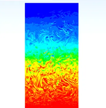
It occurs with high density fluid at the bottom and low density fluid at the top.
Why Steady State Simulation is used?
Steady state simulation is not used because it is a time independent approach. The simulation carried out here involves high turbulence and change in flow occurs in small time intervals. This is not possible to carry in steady state simulation. Moreover, the equilibrium described cannot also be captured using steady state approach.
ATWOOD NUMBER
The Atwood number (A) is a dimensionless number in fluid dynamics used in the study of hydrodynamic instabilities in density stratified flows. It is a dimensionless density ratio defined as
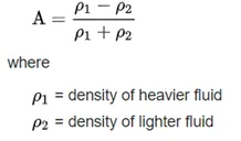
For Cases 1,2 and 3 ρair =1.225 kg/m^3 ρwater =998 kg/m^3. A= 0.997
For Case 4 ρair =1.225 kg/m^3 ρusd =400kg/m^3 A=0.42775
Effect of Atwood Number
The evolution of a uniform interface subjected to a perturbed shock wave has been experimentally studied over a range of Atwood numbers 0.22≤A≤0.68. The average bubble acceleration is nearly proportional to the square of Mach number at At = 0.9.