Week 4 - CHT Analysis on Exhaust port
AIM:- The project aim is to Conjugate Heat Transfer analysis on the Exhaust port.
OBJECTIVE:- The main objectives of our project are-
- We will give a brief description of why and where a CHT analysis is used.
- We maintain the y+ value according to the turbulence model and justify the results.
- We calculate the wall/surface heat transfer coefficient on the internal solid surface and show the velocity and temperature contours in appropriate areas.
- We verify if the HTC predictions from the simulations are right or wrong and on what factors the accuracy of the prediction depends.
PROJECT REPORT:-
Conjugate heat transfer
Conjugate heat transfer corresponds with the combination of heat transfer in solids and heat transfer in fluids. In solids, conduction often dominates whereas, in fluids, convection usually dominates. Conjugate heat transfer is observed in many situations. For example, heat sinks are optimized to combine heat transfer by conduction in the heat sink with the convection in the surrounding fluid.
Common applications and the use cases of this thermal simulation type include electronics cooling, heat exchangers, industrial machinery, some AEC cases, and more.
Heat transfer in solids and heat transfer in fluids are combined in the majority of applications. This is because fluids flow around solids or between solid walls and because solids are usually immersed in a fluid. An accurate description of heat transfer modes, material properties, flow regimes, and geometrical configurations enables the analysis of temperature fields and heat transfer. Such a description is also the starting point for a numerical simulation that can be used to predict conjugate heat transfer effects or to test different configurations in order, for example, to improve the thermal performances of a given application.
Fluid and Solid Interaction:-
The temperature field and the heat flux are continuous at the fluid/solid interface. However, the temperature field can rapidly vary in a fluid in motion: close to the solid, the fluid temperature is close to the solid temperature, and far from the interface, the fluid temperature is close to the inlet or ambient fluid temperature. The distance where the fluid temperature varies from the solid temperature to the fluid bulk temperature is called the thermal boundary layer. The thermal boundary layer size and the momentum boundary layer relative size are reflected by the Prandtl number(`Pr = (mu*C_P)/k`) for the Prandtl number to equal 1, thermal and momentum boundary layer thicknesses need to be the same. A thicker momentum layer would result in a Prandtl number larger than 1. Conversely, a Prandtl number smaller than 1 would indicate that the momentum boundary layer is thinner than the thermal boundary layer. The Prandtl number for air at atmospheric pressure and 20°C is 0.7. That is because, for air, the momentum and thermal boundary layer have similar sizes, while the momentum boundary layer is slightly thinner than the thermal boundary layer. For water at 20°C, the Prandtl number is about 7. So, in water, the temperature changes close to a wall are sharper than the velocity change.
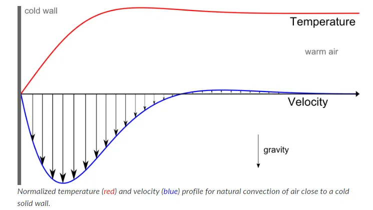
Here we do conjugate heat transfer analysis on the exhaust port. So now we go for our simulation part. We see here two casses, in our first case we take the base meshing and second case we refined our mesh and then we compare the result. We complete those simulation step by step.
CASE-1
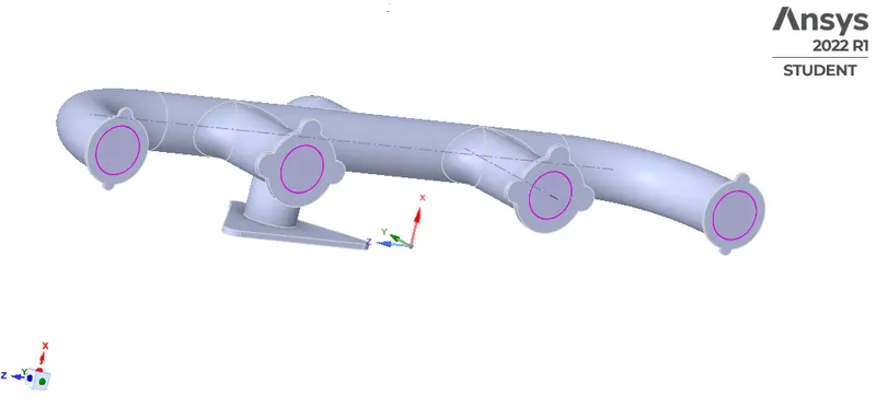
Geometry:-
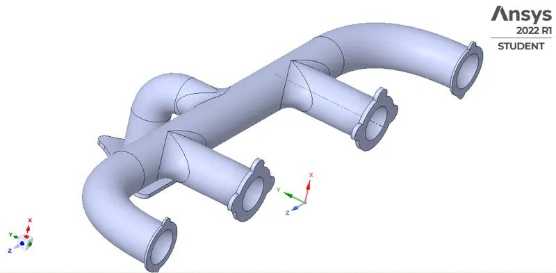
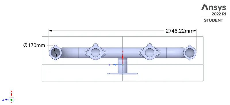
Dimension of the geometry:-
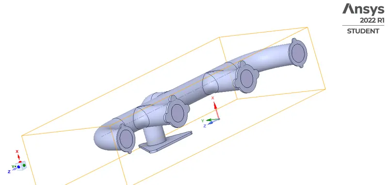
Now we need to create fluid volume, so we use volume extract option and clicking internal curve where we need the fluid.
Now we have to click on the share option in workspace since fluid and solid share the information between them:-
Meshing:-
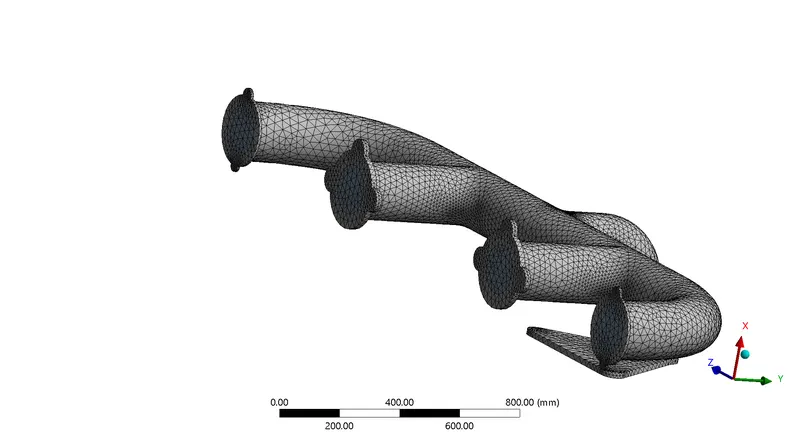
Our base meshing looks like:-
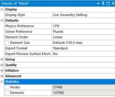
Mesh Details:-
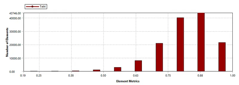
Mesh Quality:-
Named Selection:-
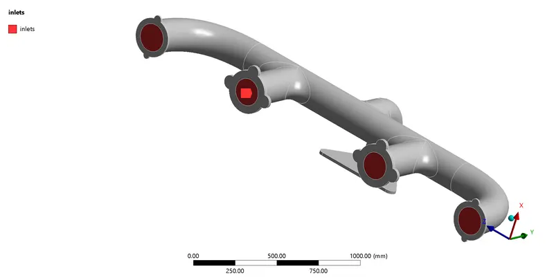
Inlets:-
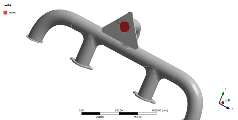
Outlet:-
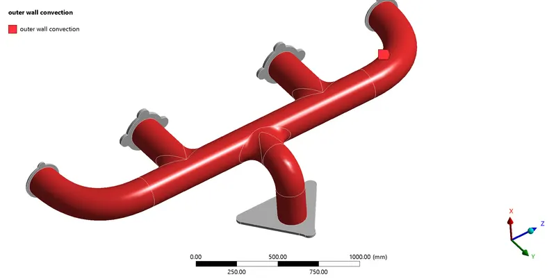
Outer wall convection:-
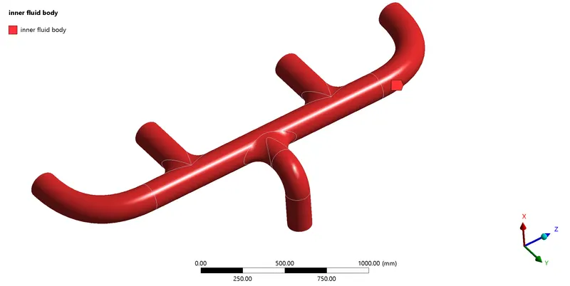
Inner body:-
Solution Report:-
Models
------

   Model                        Settings
   ---------------------------------------------------------
   Space                        3D
   Time                         Steady
   Viscous                      SST k-omega turbulence model
   Heat Transfer                Enabled
   Solidification and Melting   Disabled
   Radiation                    None
   Species                      Disabled
   Coupled Dispersed Phase      Disabled
   NOx Pollutants               Disabled
   SOx Pollutants               Disabled
   Soot                         Disabled
   Mercury Pollutants           Disabled
   Structure                    Disabled
   Acoustics                    Disabled
   Eulerian Wall Film           Disabled
   Potential/Li-ion Battery     Disabled
   Multiphase                   Disabled


Material Properties
-------------------

   Material: air (fluid)

      Property                        Units      Method     Value(s)
      ----------------------------------------------------------------
      Density                         kg/m^3     constant   1.225
      Cp (Specific Heat)              J/(kg K)   constant   1006.43
      Thermal Conductivity            W/(m K)    constant   0.0242
      Viscosity                       kg/(m s)   constant   1.7894e-05
      Molecular Weight                kg/kmol    constant   28.966
      Thermal Expansion Coefficient   K^-1       constant   0
      Speed of Sound                  m/s        none       #f

   Material: aluminum (solid)

      Property               Units      Method     Value(s)
      -----------------------------------------------------
      Density                kg/m^3     constant   2719
      Cp (Specific Heat)     J/(kg K)   constant   871
      Thermal Conductivity   W/(m K)    constant   202.4


Cell Zone Conditions
--------------------

   Zones

      name                            id   type
      ------------------------------------------
      final_geometry-solid_volume     5    solid
      final_geometry-fluid_volume_1   6    fluid

   Setup Conditions

      final_geometry-solid_volume

         Condition       Value
         ---------------------
         Frame Motion?   no

      final_geometry-fluid_volume_1

         Condition       Value
         ---------------------
         Frame Motion?   no


Boundary Conditions
-------------------

   Zones

      name                               id   type
      -------------------------------------------------------
      wall-final_geometry-solid_volume   1    wall
      inner_body                         4    wall
      inlets                             9    velocity-inlet
      outlet                             10   pressure-outlet
      outer_wall_convection              11   wall
      inner_body-shadow                  8    wall

   Setup Conditions

      wall-final_geometry-solid_volume

         Condition         Value
         ---------------------------
         Thermal BC Type   Heat Flux

      inner_body

         Condition         Value
         -------------------------
         Thermal BC Type   Coupled

      inlets

         Condition                  Value
         --------------------------------
         Velocity Magnitude [m/s]   5
         Temperature [K]            700

      outlet

         Condition   Value
         -----------------

      outer_wall_convection

         Condition                                          Value
         -------------------------------------------------------------
         Thermal BC Type                                    Convection
         Convective Heat Transfer Coefficient [W/(m^2 K)]   20

      inner_body-shadow

         Condition                  Value
         ------------------------------------------
         Thermal BC Type            Coupled
         Wall Motion                Stationary Wall
         Shear Boundary Condition   No Slip
         Wall Surface Roughness     0


Solver Settings
---------------

   Equations

      Equation     Solved
      -------------------
      Flow         yes
      Turbulence   yes
      Energy       yes

   Numerics

      Numeric                         Enabled
      ---------------------------------------
      Absolute Velocity Formulation   yes

   Pseudo Time Explicit Relaxation Factors

      Variable                    Relaxation Factor
      ---------------------------------------------
      Density                     1
      Body Forces                 1
      Turbulent Kinetic Energy    0.75
      Specific Dissipation Rate   0.75
      Turbulent Viscosity         1
      Energy                      0.75
      Explicit Momentum           0.5
      Explicit Pressure           0.5

   Linear Solver

      Variable                    Solver Type   Termination Criterion   Residual Reduction Tolerance
      ----------------------------------------------------------------------------------------------
      Flow                        F-Cycle       0.1
      Turbulent Kinetic Energy    F-Cycle       0.1
      Specific Dissipation Rate   F-Cycle       0.1
      Energy                      F-Cycle       0.1

   Pressure-Velocity Coupling

      Parameter                               Value
      -----------------------------------------------
      Type                                    Coupled
      Pseudo Time Method (Global Time Step)   yes

   Discretization Scheme

      Variable                    Scheme
      -----------------------------------------------
      Pressure                    Second Order
      Momentum                    Second Order Upwind
      Turbulent Kinetic Energy    Second Order Upwind
      Specific Dissipation Rate   Second Order Upwind
      Energy                      Second Order Upwind

   Solution Limits

      Quantity                         Limit
      ---------------------------------------
      Minimum Absolute Pressure        1
      Maximum Absolute Pressure        5e+10
      Minimum Temperature              1
      Maximum Temperature              5000
      Minimum Turb. Kinetic Energy     1e-14
      Minimum Spec. Dissipation Rate   1e-20
Maximum Turb. Viscosity Ratio 100000 Results:-
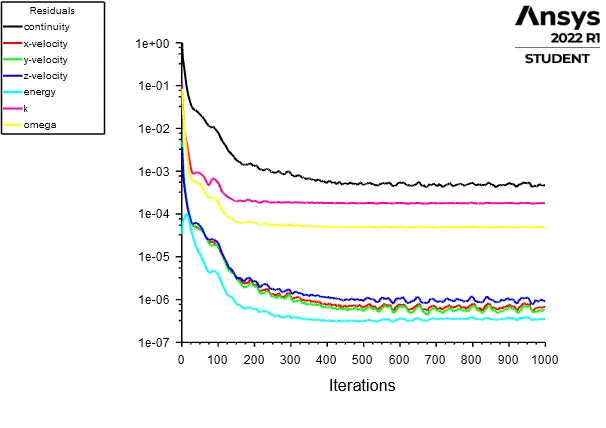
Residual:-
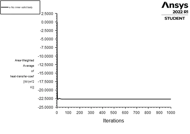
Surface Heat transfer Coefficient of inner solid body:-
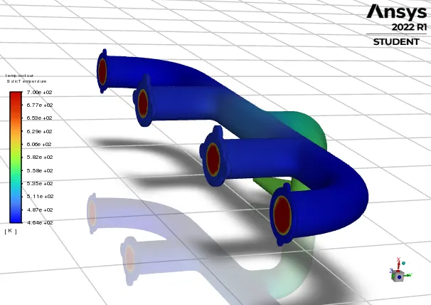
Temparature contour:-
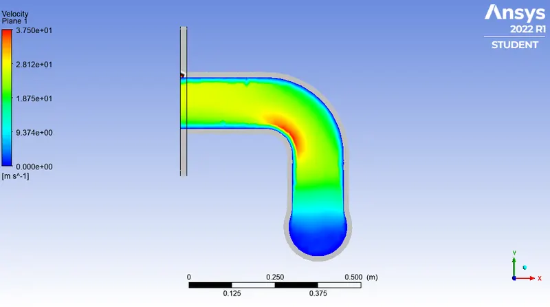
Velocity contour of xy plane:-
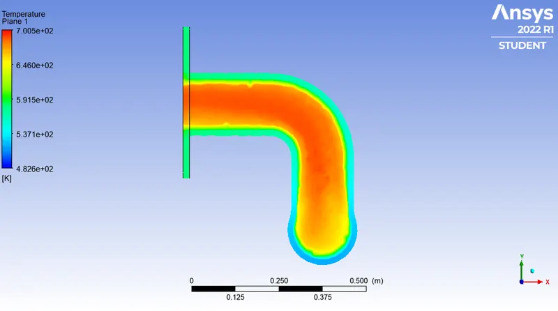
Temperature contour of xy plane:-
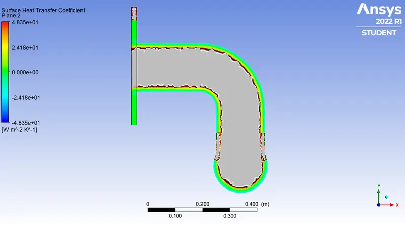
S-htc contour of xy plane:-
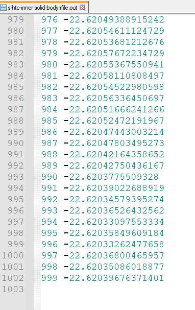
Surface heat transfer coefficient value in different iteration:-
Case-2:- Here first we prepare geometry same as the base simulation. So we do not repeat those process again instead we go for meshing.
Meshing:- After doing the base meshing we add inflation layer to accurately calculate surface heat transfer coefficient value for inner solid body part.
Inflation layer:-
In setting up cases for Reynolds averaged Navier-Stokes (RANS) analysis for CFD, we usually incorporate a prism layer along wall surfaces to capture boundary later effects in better detail. The technique in such cases would be to size the first layer of mesh for a target y+ value.
Since we are more aware of heat transfer near the wall which is under the viscous sublayer, so we have to take the Y+ value between 1 to 5. We take the Y+ value as 1. Now we have to calculate the first layer thickness and to do that we first calculate the Reynolds number using the following equation
Re = `(ρVd)/μ` , where `ρ` is the density of the fluid, V is the fluid velocity, d is the inlet diameter of the exhaust port and `μ` is the viscosity of the fluid.
The value of `rho` = 1.225,`mu` = 1.7894e-05, V = 5, D = 0.17 m. SO,
Re = `(1.225 * 5 * 0.17)/(1.7894e-05)` = 58189.9
Skin friction coefficient, C_f = `0.079/(Re^0.25) = 5.086*10^-3`
Wall shear stress, tau_w = `½*C_f*rho*V^2` = 0.0779 PaFrictional velocity, U_T = `√(τ_w/ρ)` = `√((0.0779/1.225) )` = 0.252 m/s.
Now, we know Y+ = `(ρ*U_T*∆y_1)/μ` , where is the first-layer thickness of the inflation layer.So, =`(Y+ * μ) / (ρ*U_T)`= (1*1.7894e-05) / (1.225*0.252) = 5.796e-05 m = 5.796e-02mm
So, the total thickness = `("First layer thickness")*[1-g^(N+1)]/(1-g)`
Where g is growth rate and N is number of layers
= `5.796e-02*[1-1.2^7]/(1-1.2)`
= 74.86e-02mm
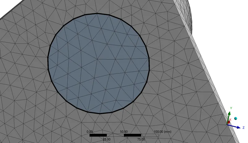
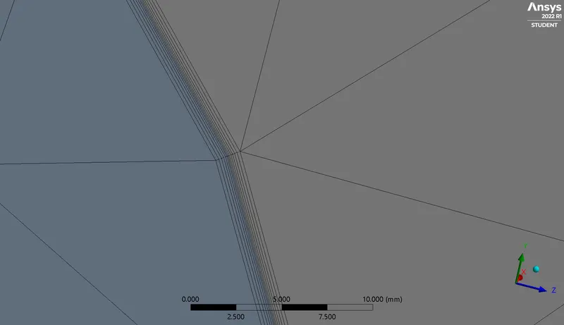
After addding the inflation layer we give the solid body mesh size 0.18 mm. And now the geometry looks like-
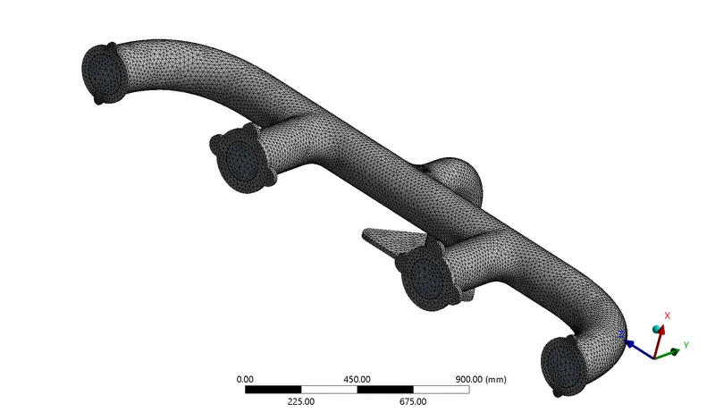
Mesh Details:-
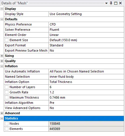
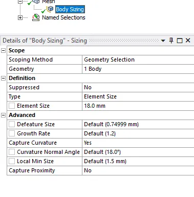
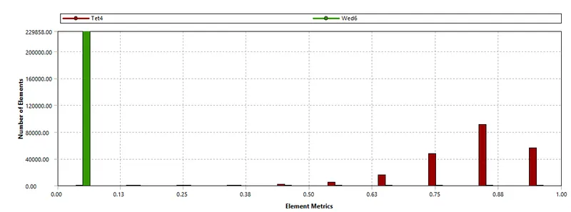
Checking Mesh Quality:- By seeing the plots, we can say that our mesh is good enough to give a better result.

Results:-
Solution Report:-
Models
------

   Model                        Settings
   ---------------------------------------------------------
   Space                        3D
   Time                         Steady
   Viscous                      SST k-omega turbulence model
   Heat Transfer                Enabled
   Solidification and Melting   Disabled
   Radiation                    None
   Species                      Disabled
   Coupled Dispersed Phase      Disabled
   NOx Pollutants               Disabled
   SOx Pollutants               Disabled
   Soot                         Disabled
   Mercury Pollutants           Disabled
   Structure                    Disabled
   Acoustics                    Disabled
   Eulerian Wall Film           Disabled
   Potential/Li-ion Battery     Disabled
   Multiphase                   Disabled


Material Properties
-------------------

   Material: air (fluid)

      Property                        Units      Method     Value(s)
      ----------------------------------------------------------------
      Density                         kg/m^3     constant   1.225
      Cp (Specific Heat)              J/(kg K)   constant   1006.43
      Thermal Conductivity            W/(m K)    constant   0.0242
      Viscosity                       kg/(m s)   constant   1.7894e-05
      Molecular Weight                kg/kmol    constant   28.966
      Thermal Expansion Coefficient   K^-1       constant   0
      Speed of Sound                  m/s        none       #f

   Material: aluminum (solid)

      Property               Units      Method     Value(s)
      -----------------------------------------------------
      Density                kg/m^3     constant   2719
      Cp (Specific Heat)     J/(kg K)   constant   871
      Thermal Conductivity   W/(m K)    constant   202.4


Cell Zone Conditions
--------------------

   Zones

      name                                                  id   type
      ----------------------------------------------------------------
      final_geometry-final_geometry_solid_volume            5    solid
      final_geometry-final_geometry_fluid_volume_1_volume   6    fluid

   Setup Conditions

      final_geometry-final_geometry_solid_volume

         Condition       Value
         ---------------------
         Frame Motion?   no

      final_geometry-final_geometry_fluid_volume_1_volume

         Condition       Value
         ---------------------
         Frame Motion?   no


Boundary Conditions
-------------------

   Zones

      name                                              id   type
      ----------------------------------------------------------------------
      wall-final_geometry-final_geometry_solid_volume   1    wall
      inner_fluid_body                                  4    wall
      inlets                                            9    velocity-inlet
      outlet                                            10   pressure-outlet
      outer_wall_convection                             11   wall
      inner_fluid_body-shadow                           8    wall

   Setup Conditions

      wall-final_geometry-final_geometry_solid_volume

         Condition         Value
         ---------------------------
         Thermal BC Type   Heat Flux

      inner_fluid_body

         Condition         Value
         -------------------------
         Thermal BC Type   Coupled

      inlets

         Condition                  Value
         --------------------------------
         Velocity Magnitude [m/s]   5
         Temperature [K]            700

      outlet

         Condition   Value
         -----------------

      outer_wall_convection

         Condition                                          Value
         -------------------------------------------------------------
         Thermal BC Type                                    Convection
         Convective Heat Transfer Coefficient [W/(m^2 K)]   20

      inner_fluid_body-shadow

         Condition                  Value
         ------------------------------------------
         Thermal BC Type            Coupled
         Wall Motion                Stationary Wall
         Shear Boundary Condition   No Slip
         Wall Surface Roughness     0


Solver Settings
---------------

   Equations

      Equation     Solved
      -------------------
      Flow         yes
      Turbulence   yes
      Energy       yes

   Numerics

      Numeric                         Enabled
      ---------------------------------------
      Absolute Velocity Formulation   yes

   Pseudo Time Explicit Relaxation Factors

      Variable                    Relaxation Factor
      ---------------------------------------------
      Density                     1
      Body Forces                 1
      Turbulent Kinetic Energy    0.75
      Specific Dissipation Rate   0.75
      Turbulent Viscosity         1
      Energy                      0.75
      Explicit Momentum           0.5
      Explicit Pressure           0.5

   Linear Solver

      Variable                    Solver Type   Termination Criterion   Residual Reduction Tolerance
      ----------------------------------------------------------------------------------------------
      Flow                        F-Cycle       0.1
      Turbulent Kinetic Energy    F-Cycle       0.1
      Specific Dissipation Rate   F-Cycle       0.1
      Energy                      F-Cycle       0.1

   Pressure-Velocity Coupling

      Parameter                               Value
      -----------------------------------------------
      Type                                    Coupled
      Pseudo Time Method (Global Time Step)   yes

   Discretization Scheme

      Variable                    Scheme
      -----------------------------------------------
      Pressure                    Second Order
      Momentum                    Second Order Upwind
      Turbulent Kinetic Energy    Second Order Upwind
      Specific Dissipation Rate   Second Order Upwind
      Energy                      Second Order Upwind

   Solution Limits

      Quantity                         Limit
      ---------------------------------------
      Minimum Absolute Pressure        1
      Maximum Absolute Pressure        5e+10
      Minimum Temperature              1
      Maximum Temperature              5000
      Minimum Turb. Kinetic Energy     1e-14
      Minimum Spec. Dissipation Rate   1e-20
      Maximum Turb. Viscosity Ratio    100000
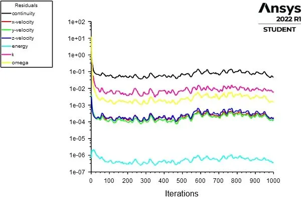
Residual:-
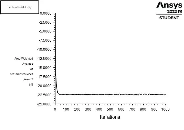
Surface heat transfer coefficient of internal solid surface:-
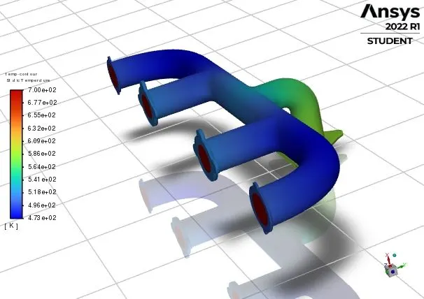
Temparature contour:-
Velocity Stramline:-
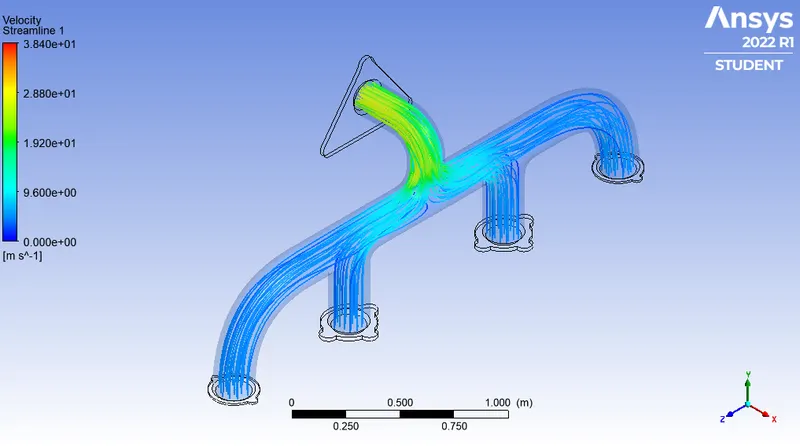
Velocity Stramline:-
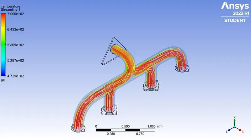
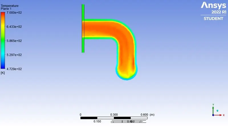
Temparature contour of xy plane:-
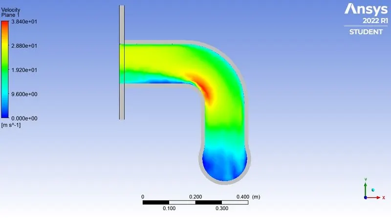
Veklocity contour of xy plane:-
S-htc contour of xy plane:-
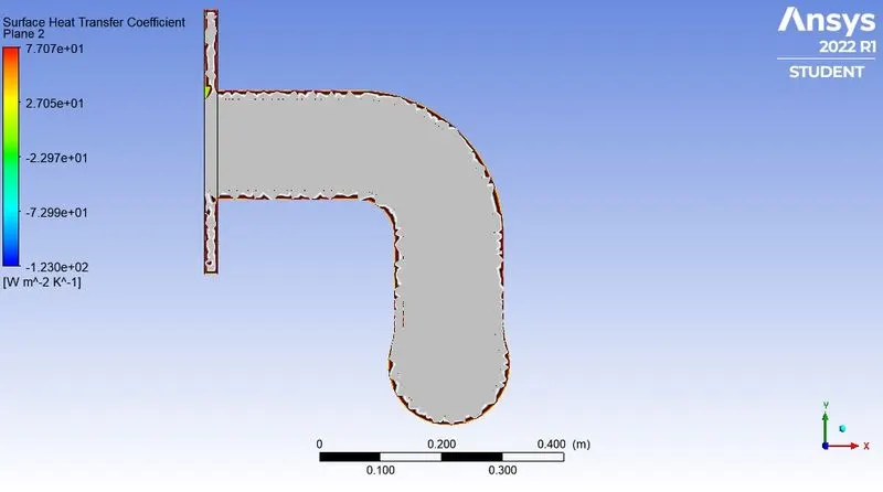
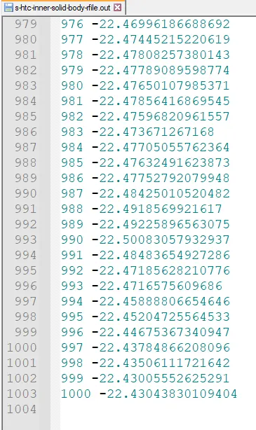
Surface heat transfer coefficient value in different iteration:-
Analytical solution for Heat transfer coefficient:-
The Reynolds number of the flow is 58189.9 which means the flow is turbulent.
Prandtl number, `Pr = (mu*C_P)/k`
Where `mu` si the dynamic viscosity of the fluid = 1.7894e-05 kg/m-sec
k, is the thermal conductivity of the material, = 0.0242 W/mK
`C_p` is the specific heat capacity of the fluid at constant pressure = 1006.43 J/kg-K
Therefore, Pr = `(mu*C_p)/k` = `(1.7894e-05*1006.43)/0.0242` = 0.744
The length of the manifold, L = 2746.22, The diameter, D = 170
So,`L/D = 2746.22/170` = 16.15 >10
The local Nusselt number may be obtained from the well-known Dittus-Boelter equation. The Dittus-Boelter equation is easy to solve.
Correlation: Dittus-Boelter
`Nu_(Dh) = 0.023*RE_(Dh)^0.8*Pr^0.4`
Where: Dh is the hydraulic diameter[m],
Re is the Reynolds number,
Pr is the Prandtl number,
Nu is the Nusselt number.
This equation is validated for
- 0.6 <= Pr <= 160
- Re_Dh > 10000
- L/D > 10
In our case, all the conditions are valid for the Dittus Boelter equation. So, we can apply this equation to calculate the Nusselt number. So,
Nu_Dh = 0.023*RE_Dh^0.8* Pr^0.4
= `0.023*(58189.9^0.8)*(0.744^0.4)` = 132.5
We also know that, `Nu_(Dh) = (h*D)/k` [Here, h = heat transfer coefficient]
Heat transfer coefficient, `h = (Nu_(Dh)*k)/D`
= `(132.5*0.0242)/0.17`
= 18.86 `W/(m^2K)`
The accuracy of the prediction depends on:-
- The number of elements in the mesh is an important factor to bring accuracy to the result.
- The accuracy of the heat transfer coefficient depends on selecting the suitable value of Y+ and the right turbulence model. Selecting the right turbulence model is a difficult thing. The eight RANS turbulence models differ in how they model the flow close to walls, the number of additional variables solved for, and what these variables represent. All of these models augment the Navier-Stokes equations with an additional turbulence eddy viscosity term, but they differ in how it is computed.
OBSERVATION:-
Surface heat transfer coefficient value for case-1 is 22.62 `W/(m^2*k)`, and for case-2 means refined case s-htc value is unsteady means it's changing with time but we take the value of last iteration which is -22.43 `W/(m^2*k)`
Observation table:-
| Number of casses | Number of cells | First layer thickness | Number of inflation layer | Analytical Value of S-HTC | Numerical value of S-HTC | Error |
| case-1 | 137992 | NA | NA | 18.86 `W/(m^2K)` | 22.62 `W/(m^2K)` | 3.76 |
| case-2 | 445069 | 0.74mm | 6 | 18.86`W/(m^2K)` | 22.43 `W/(m^2K)` | 3.57 |
CONCLUSION:- At last we have done our simulation successfully, so now we conclude our results-
- Finner mesh gives the more accurate result and more accurate plots which we see here.
- The accuracy of the heat transfer coefficient depends on selecting the suitable value of Y+ and the right turbulence model. Here we select the Y+ value as 1 and the turbulence model as the k-`omega` sst model.
- If we see the results, the fluid flow velocity through inlets is near zero compared to fluid flow velocity through outlet is much higher.
- There are 4 inlets and 1 outlet in the manifold, so through the outlet more fluid is transferred and that's why more temperature is transferred from the fluid to the solid in the outlet section.
- The value of the Surface heat transfer coefficient is unsteady means its value is changing with time.
- Always we have to compare our result with the analytical value to check how much accurate our result is.