Week 4 - CHT Analysis on Exhaust port
1.Aim:
Steady state CHT analysis on Exhaust port at an inlet velocity of 5 m/s.
2.Introduction:
Simulate fluid flow and assume that the walls of the container were at a constant temperature or even adiabatic. In reality, however, the heat transfer between solids and surrounding fluids couples the temperature field in both materials, and thus your CFD software must be able to account for this phenomenon. CONVERGE features a state-of-the-art conjugate heat transfer (CHT) model for simultaneously predicting heat transfer in both the fluid and solid portions of the domain, which is critical for many applications.
2.1 Conjugate Heat Transfer
- Conjugate heat transfer problem is a coupled, fluid-structure, heat transfer problem where conduction heat transfer in a solid wall interacts with fluid flow and the convection heat transfer in fluid flow interacts at the solid boundary. Fluid network modeling with conjugate heat transfer has many applications.
- The Conjugate Heat Transfer analysis type allows for the simulation of heat transfer between solid and fluid domains by exchanging thermal energy at the interfaces between them.
- The finite volume formulation requires governing equations to be expressed in conservative form. The rate of change of a conserved property in a given control volume is expressed as the vector sum of transported property from neighboring control volumes together with source or sink terms. The unknown variables in the flow circuit of pressure, temperatures of fluid and solid and flowrate.
2.2 Application
-
Wall temperature is a function of flow, a coupled analysis of temperature of solid and fluid is necessary. In cryogenic applications, such as medical and space technology, modeling of conjugate heat transfer is of great importance. In space technology applications, correct prediction of boil-off rate in propellant tanks and chilldown of Hitrogen, Nitrogen and etc.
2.3 Steps involves in Ansys Fluent software
- Geometry: Construct a two or three dimensional representation of the object to be modelled and tested using the work plane co-ordinate system within Ansys.
- Mesh: At this point understands the makeup of the part. Now define how the modelled system should be broken down into finite pieces.
- Setup: This case setup will be done using Ansys Fluent.
- Solution: Ansys Fluent where run time result visualization is done.
- Results: Post processing of results will be done using CFD post.
3.Procdure:
3.1 Geomentry
1.Open new project, by clicking on Fluid flow(Fluent) in Ansys workbench.
2.Now click on geometry to import exhaust port. It will redirect to Spaceclaim, Ansys geometry model. 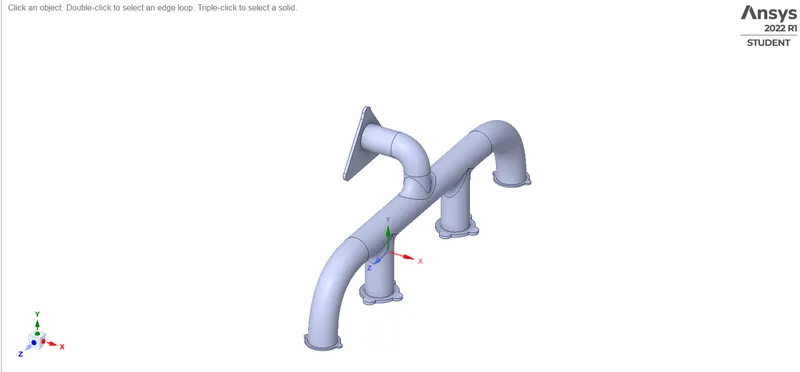
Fig: Exhaust port
3.We are to analyse the mixing of two fluid, SO there is role of part other than two pipes. To supress that we need to extract edge of port. Go to prepare menu and click on volume extract. Switch to edge selection and select five outer edges and click on green check button
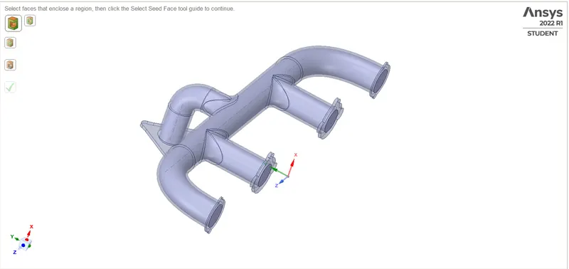
Fig: Extracted port model
4.Moving the 2 volume and create new volume and select the fff body make to delete the empty volume
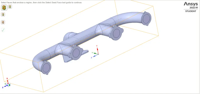
Fig: New volume
5. Now select the share topology
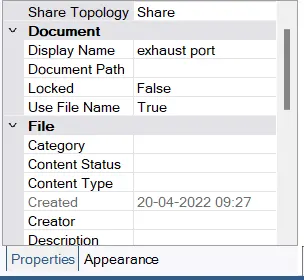
Fig: Share Topology
6.For a Good quality mesh interference, select workbench > share the entire body ( That pink colour shows the bodies are interference)
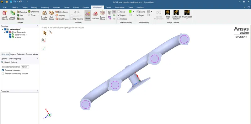
Fig: Bodies interference
7.Exit from Spaceclaim and click on mesh to open mesh menu.
3.2 Mesh
8.Select wall face and press right click of mouse, it will open a menu. Click on option create named selection and write suitable name for face. Repeat for other faces.
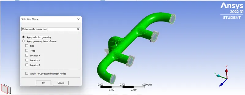
Fig: Selection Name Menu
9. Now click on mesh option and choose generate mesh. It will generate mesh Initial mesh.
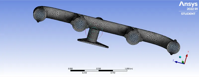
Fig: Initial Generated Mesh
10. Inflation sizing:
This option is used to accurately capture the boundary layers on the surface of the port.
First layer thickness=0.005m
Incremental ratio = 1.2 times of previous layer (or) 20% of previous layer
Total layer and Total thickness in this problem = 5 layers and 0.0005m.
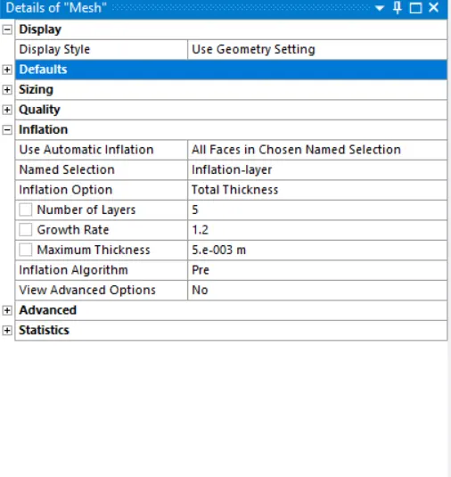
Fig: Inflation sizing
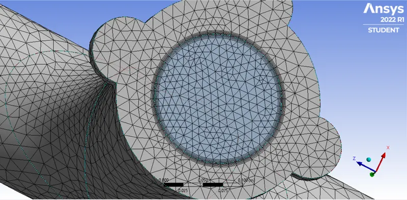
Fig: Inflation layer
11.Body sizing: This option is used to refine the layer inner enclosure of the wind tunnel. The increased size gives us more accurate results near the Exhaust port. Element size 0.01m
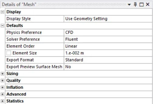
Fig: Body sizing
3.3 Setup and Solution
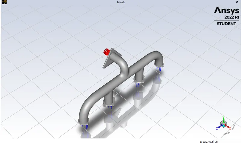
Fig: Exhaust port
12.Exit mesh and open setup. First, Check mesh, it is throwing no error then only we can proceed further. We are going to do pressure based steady state simulation, So choose these options on task page.
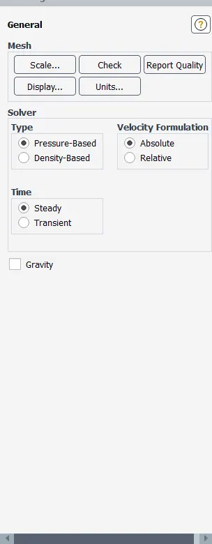
Fig: Task page
13. Go to physics menu and select viscous model. It will open a menu, choose realizable K-omega model and close it.
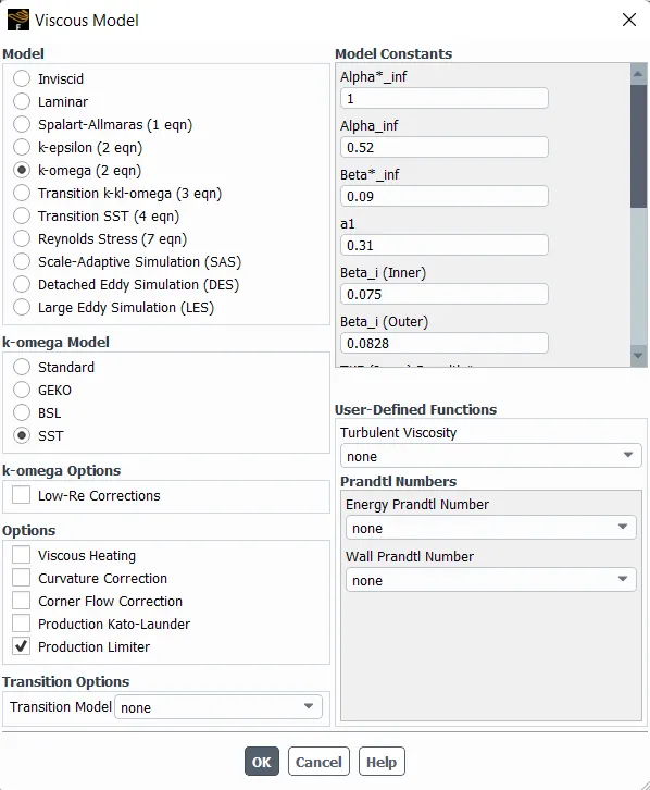
Fig: Viscous model parameters
14.Click on material and choose air as working fluid. check working fluid by clicking on cell zone conditions option, if it Fluid is air & Solid is aluminum then proceed.
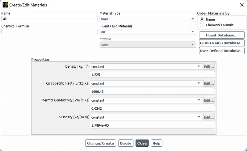
Fig: Fluid Mateials
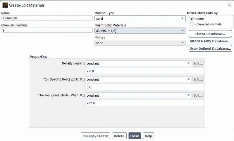
Fig: Solid materials
15.Now go to boundaries option to set boundary conditions. Select inlet x and click on option edit. It will open a menu, Where it is thermal radiation, momentum etc. Put the value of velocity as 5 m/s and go to thermal parameter to set temperature as 700k.
16.Now click on intialization to calculate approximate values of velocity and pressure.
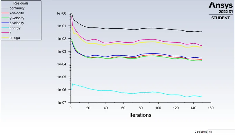
17.Change the number of iteration 160 and click on calculate.
18.Exit setup and double click on result to open CFD post. Check boxes to see walls and other parts.
4.Results
Residual
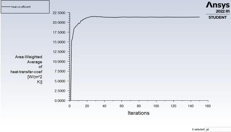
Surface Heat Transfer Co-efficient
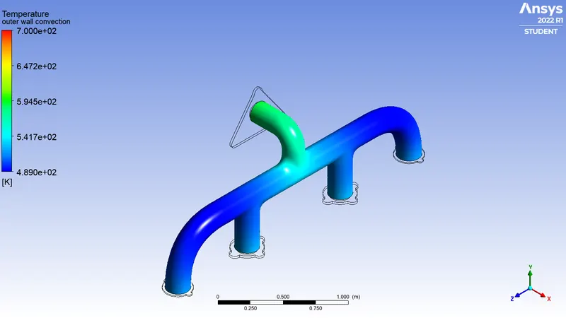
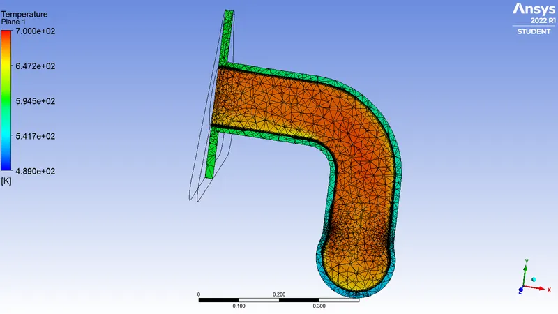
Tmeperature contour
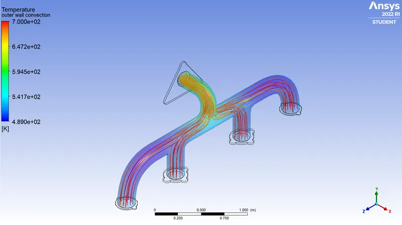
Temperature contour with Streamlne
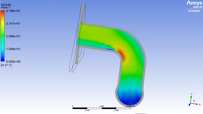
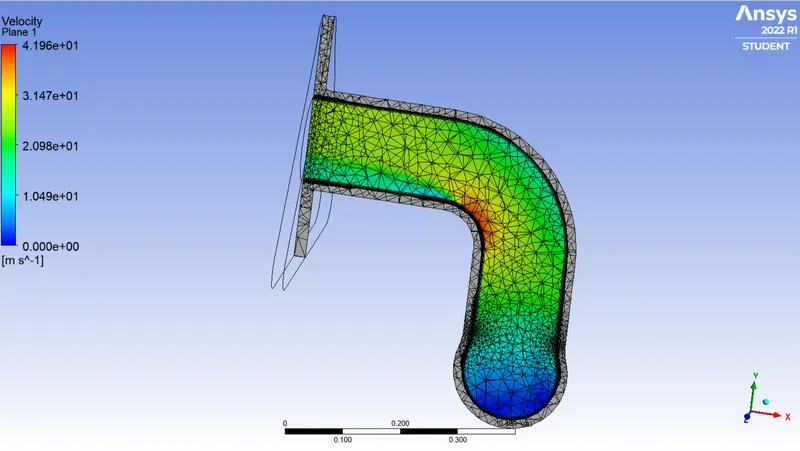
Velocity of Outlet plane
Velocity of Outlet plane with Mesh
Temperature of Outlet plane
5.Grid Dependancy:
A Grid Dependance Test is used to as certain whether the final values of the solution are dependent on the mesh or not. This is an important test to ensure the simulation results are correct.
5.1 Analytical solution
The Reynolds number for the given flow is 58189.89 Which suggests that the flow is turbulent in nature,the Dittus bolter heat transfer co-efficient relation can be used to determine the Nusselt number which is described mathematically as follows
Nu(D) = 0.023*Re^(3/4)*Pr^n
where Pr = (μ*Cp)/k
μ= 1.17894e-05 (kg/m-sec)
k=0.0242 (W/mK)
Cp=1006.43 (J/kgK)
Pr = (μ*Cp)/k = (1.17894e-05 * 1006.43)/0.0242
Pr= 0.744, n is constant =0.33
Therefore
Nu(D) = 0.023*58189.89^(3/4)*0.744^0.33 = 136.482
Therefore Convective heat transfer co-efficient
h=(Nu*k)/D
h=19.428 W/(m^2K)
| Mesh quality(m) | Body sizing(m) | Inflation sizing(m) | Number of Nodes | Number of Elements | Heat Transfer co-efficient | |
| 1st Refindment | 0.01 | 0.005 | 0.0005 | 98937 | 282008 | 21.567 |
| 2nd Refindment | 0.008 | 0.005 | 0.0005 | 106632 | 308728 | 21.235 |
| 3rd Refindment | 0.0075 | 0.004 | 0.00045 | 109478 | 319449 | 20.873 |
6.Conclusion
- Conjugate heat analysis can accurately predict heat transfer by simultaneous solving all the relevent solid and fluid field heat transfer process like free and forced convection in gases , in IC engine analysis, conduction through etc. In this study CHT analysis has done to find out temperature rise manifold because of hot air passing through it and we predicted heat transfer co-efficient as well.
- Velocity contour were created to get in sights of fluid path and maximum velocity area. It can be seen from graph that heat transfer co-efficient is related to wall only. Simulation is conducted two different mesh distinguished in size. The simulation can be performed for a wider range of base mesh size values.
- Decreasing the mesh size, the average Heat Transfer co-efficient are starts approaching towards the analytical results.