Week 4 - CHT Analysis on Exhaust port
Aim
Conjugate Heat transfer (CHT) analysis on Exhaust Port
Objectives
- A brief description of why and where a CHT analysis is used
- Maintain the y+ value according to the turbulence model and justify the results.
- Calculate the wall/surface heat transfer coefficient on the internal solid surface & show the velocity & temperature contours in appropriate areas.
- How would you verify if the HTC predictions from the simulations are right? On what factors does the accuracy of the prediction depend on?
Methodology
- Introduction
- What is Conjugate Heat Transfer (CHT) Analysis and where is it used.
A CHT analysis is nothing but an analysis where we will be modeling both the fluid flow and the heat transfer through it. Examples are, flow through the exhaust port of an engine, heat exchangers, cooling of electronic equipment, etc.
It is used to simulate the heat transfer either between solid and solid or solid and fluid.
- Why a CHT analysis is used.
In CHT analysis the wall heat transfer coefficients and other heat transfer parameters are directly calculated on the surface within the model.
- Preprocessing
- Model creation (For Baseline Meshing)
We have a solid model of the exhaust port of an inline engine from which we will extract the fluid volume and then will model both fluid flow and solid heat transfer through it.
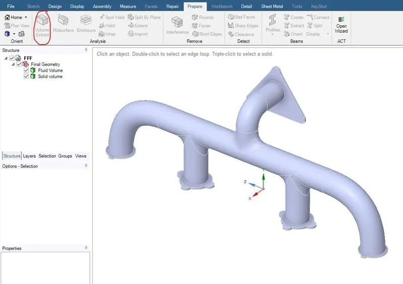
The geometry has been imported into the Spaceclaim and the inside volume is extracted using the volume extract feature in Ansys Spaceclaim under prepare tab. After extracting the volume, we will name it as fluid volume and the outer wall is named as solid volume and moved both to the new components.
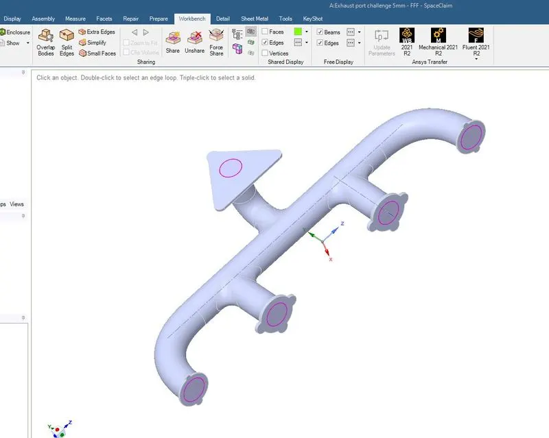
In order to be sure that the information from one region is transferred to the other region smoothly, we need to share the topology in SpaceClaim. If we don’t do this, there is a high chance that the mesh will fail.
For this go to workbench and click on share. After clicking on tick we can see a red circle at the interfaces, which says that the information’s are shared with each other.
- Naming and meshing of domains
After naming all the faces and walls we will proceed to mesh
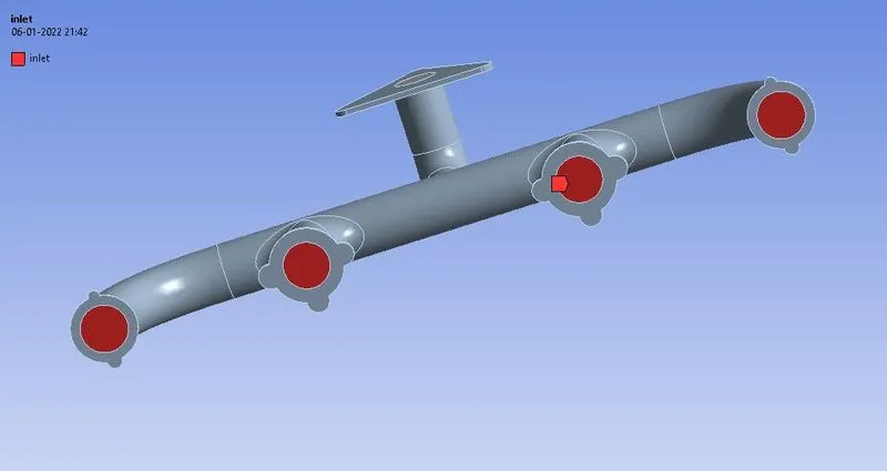
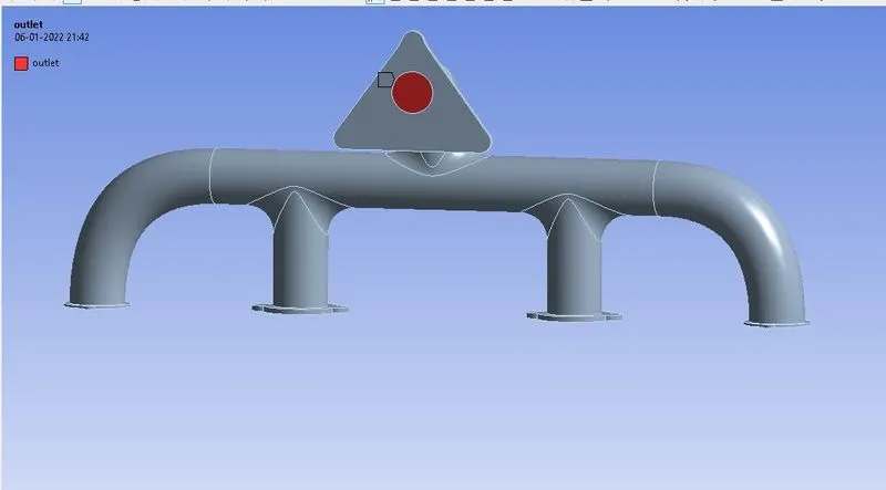
Here, we have 4 inlets, 1 outlet, 1 convective layer, and an inflation layer (for creating an inflation layer) as shown in the figures.
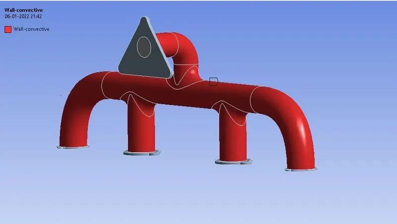
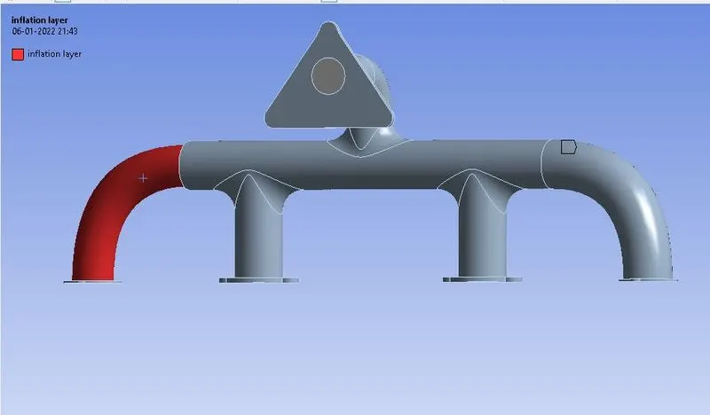
Now right-click on mesh and click on generate mesh to create baseline Mesh.
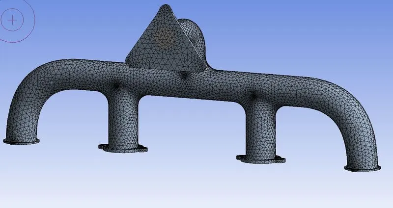
Number of elements = 136678
- Setting up the problem
Here we set up the problem by applying relevant
- Initial conditions
- Boundary conditions
- Material properties
- Turbulence Models
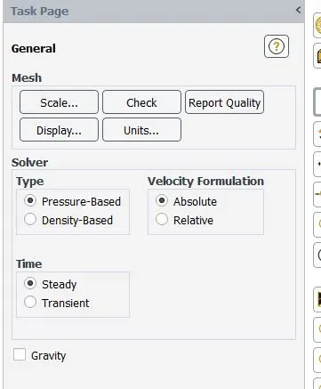
Here we are using a pressure-based (Mach number is less than 0.3) steady solver. The fluid is air with a freestream velocity of 5m/s.
- Material Properties
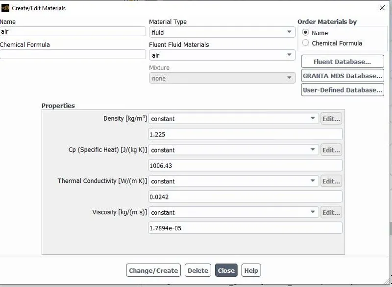
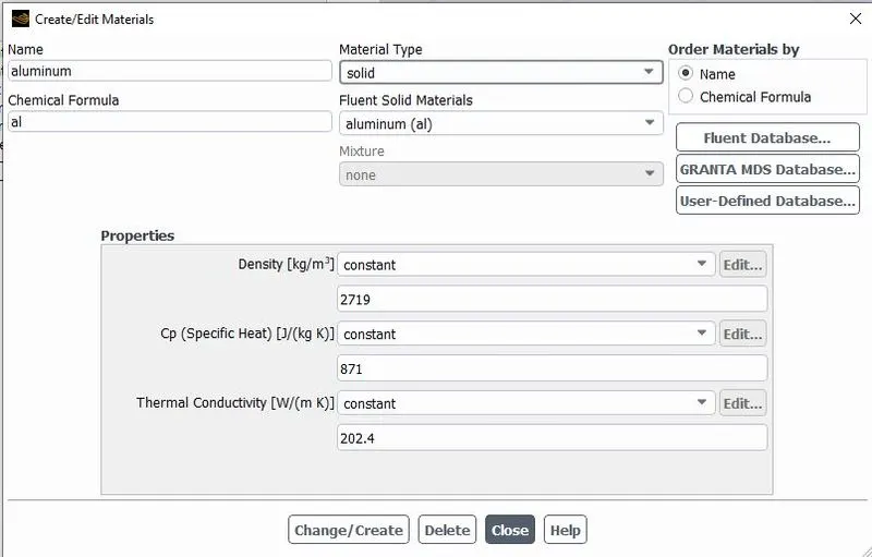
The fluid is Air and the solid is Aluminium. Material properties are as shown below.
Air Properties
Density = `1.225 (kg)/m^3`
Kinematic viscosity = `1.7894*10^-05 (kg)/(ms)`
Aluminium properties
Density =`2719 (kg)/m^3`
Thermal conductivity =`204 W/(m K)`
Turbulence Model
Reynolds number Re = `(ρ*u*l)/μ = (1.225*5*0.16611)/(1.7894e-5)=56858.37`
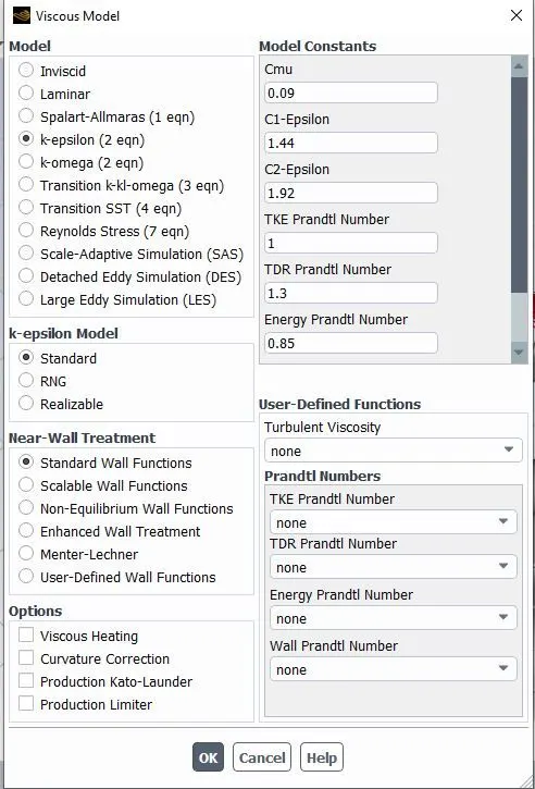
Since Reynolds number is greater than 4000 (Internal flow) the flow is turbulent. There we are using turbulence model as K-epsilon with standard wall functions.
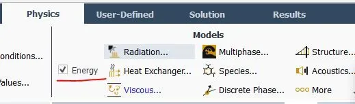
Since Temperature is involved, Energy is turned on
Initial and boundary conditions
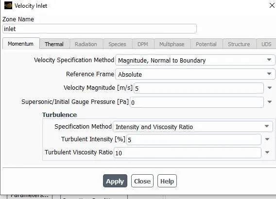
Inlet - Velocity boundary condition: Here the velocity magnitude is 5m/s
Temperature = 700 K
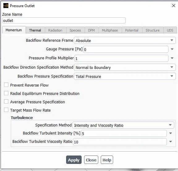
Outlet - Pressure outlet: Gauge pressure = 0
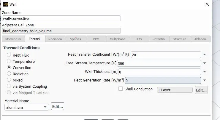
Wall-convective – Wall: convective; `h = 20 W/(m^2 K`
Symmetry wall - Symmetry
Reference Values
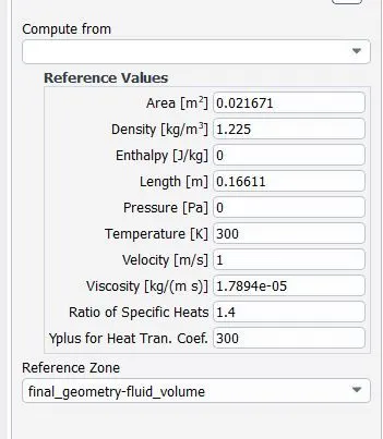
In order to get the correct drag coefficient, giving the correct reference values are very important. The following reference values have been used throughout the simulation.
Click on reference values under physics. Click on the inlet in the compute from the dropdown. Ensure that the area, density, velocity, and viscosity are as per our values. The area is nothing but the cross-sectional area in internal flows.
Result extraction
Before running the simulation let’s set up some plots and curves for extracting results as the simulation proceed. As we are interested in the temperature distribution and heat transfer properties we will take a contour plot while the program is running. Before this, initialize the solution using hybrid initialization. Then go to results and create a new contour plot for temperature.
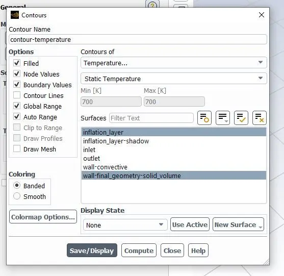
After creating temperature contour, run the simulation for 250 iterations.
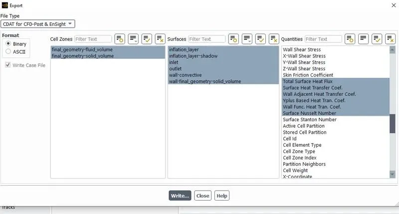
Extracting heat transfer properties: In order to plot the heat transfer coefficient on the inflation, we need to export the solution data’s to a CDAT file to visualize the coefficient of heat transfers in a plot in the CFD post. By default, these options are not available in the CFD post. That’s why we are exporting the solution data to a file.
After the simulation is over go to file then export and click on solution data.
Select CDAT for CFD-Post & EnSight as file type. Then, select all cell zones and all surfaces. After this select the required quantities that need to be exported as shown in the figure.

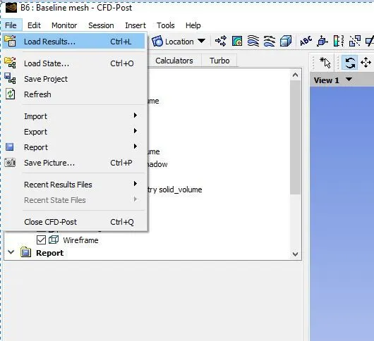
Now go to CFD Post and load the saved results by clicking on file then load results. Now the saved data will load and we can plot the required quantities as we need.
- Model creation (With local refinement)
In the above section, we created an unrefined mesh which resulted in many distorted results. In order to get a better result, we will add an inflation layer with y+ = 50.
- Naming and meshing of the domain
Naming is the same as baseline.
Let’s create an inflation layer near the fluid and wall interference region (Named it as inflation layer). As we are taking the k-epsilon turbulent model, we can take y+ in between 30 to 300. For the current cross-section let’s take y+ = 50.
Go to the properties of mesh, there we will see inflation, under inflation change use automatic inflation to All Faces in Chosen Named Selection. Select inflation layer. Change inflation options to total thickness. A number of layers = 5. The total thickness is calculated from the First layer thickness. The first layer thickness is calculated from the y+ value.
The equation for first layer thickness `y= (y^+ μ)/(ρu_t )`
Where, `u_t= √τ_w/ρ` =frictional velocity
Here `u_t` can be calculated from wall shear stress `τ_w` which is again a function of skin friction drag coefficient `C_f.`
`C_f=0.079(Re)^(-0.25)` For internal flow.
Reynolds number Re = `(ρ*u*l)/μ = (1.225*5*0.16611)/(1.7894e-5)=56858.37`
`C_f=0.079Re^(-0.25)=5.116e-3`
`τ_w= 1/2 C_f ρ〖U_∞〗^2`
`τ_w= 1/2*5.116*10^(-3)*1.225*5^2=0.07834`
`u_t= √(τ_w/ρ)= √((0.07834)/(1.225))=0.2529 m/s`
`y= (y^+ μ)/(ρu_t )= (50*1.7894*10^(-5))/(1.225*0.2529)=2.888*10^(-3) m`
Therefore First layer thickness = 2.888 mm
Hence total thickness =`2.888*(1-1.2^5)/(1-1.2)=21.5mm`
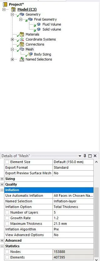
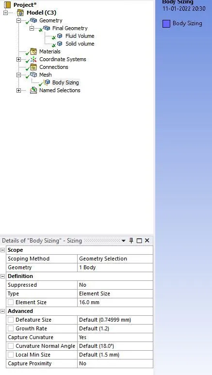
We will refine the fluid region to get a well-refined flow region. Right-click mesh click on Sizing and select fluid wall as the body. Change Element Size to 16mm. Then click on update to generate the mesh.
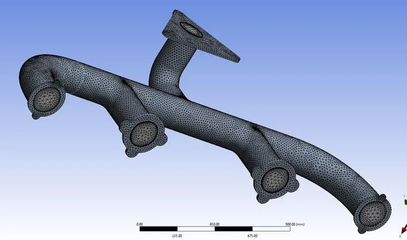
Total number of elements = 407395
The solution setup is the same as the baseline setup. After following the same steps run the simulation for 250 iterations.
- Postprocessing
- Solutions: Baseline meshing
- Residual plot
- Solutions: Baseline meshing
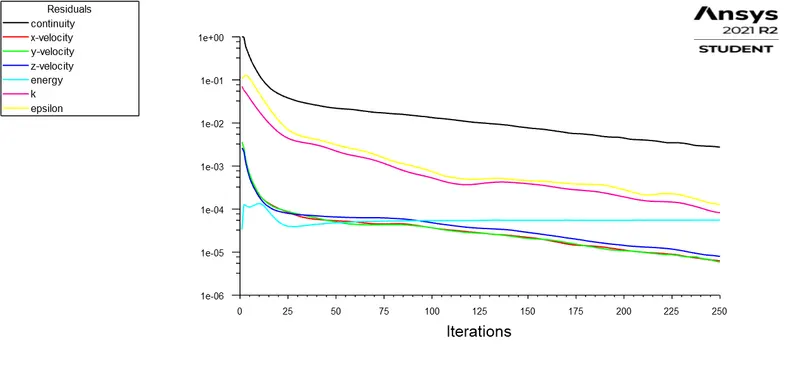
The solution is converged
- Temperature contour
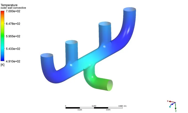
From the above temperature contour, we can observe that the temperature on the wall is getting higher as the flow approaches the exit. The velocity profile will explain the reason behind this,
- Velocity plot
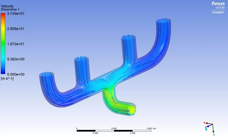
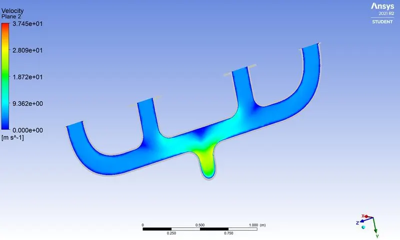
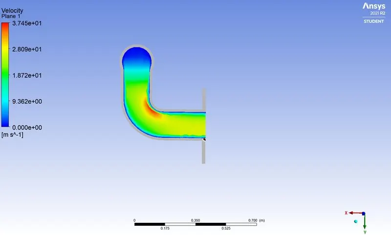
The first figure shows the streamlines inside the pipe and the other two show the velocity contours at different cross-sections to understand the temperature phenomenon.
It is seen from the plots that the velocity is increased when the flow is at the exit. The velocity is maximum for the bend near the exit. This is because of the continuity equation.
The cross-section is almost the same everywhere, hence as per the continuity equation, the mass flow rate needs to be conserved. Here in this problem, the hot fluid is entering the pipe from 4 inlets and it exits one inlet at a time. Therefore in order to match up the incoming flow rate, the flow has to increase the flow velocity. That’s why the velocity is maximum at the bend.
If the velocity is increasing, the Reynolds number increases, and eventually the temperature will increase. Hence more heat transfer near the exit.
- Surface heat transfer coefficient
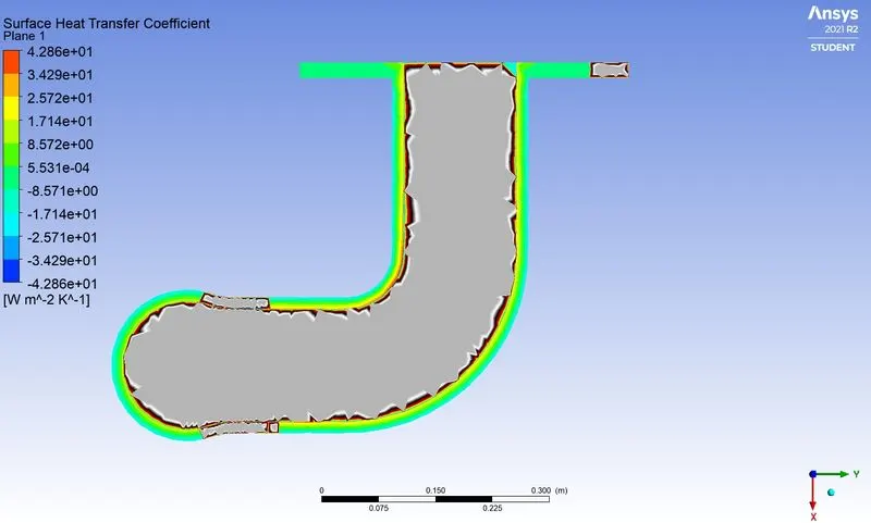
Surface heat transfer coefficient = -22.527877
- Solutions: Refined meshing
- Residual plot
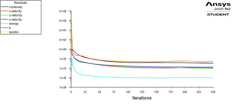
The solution is converged
Temperature contour
From the above temperature contour, we can observe that the temperature on the wall is getting higher as the flow approaches the exit. The velocity profile will explain the reason behind this,
- Velocity plot
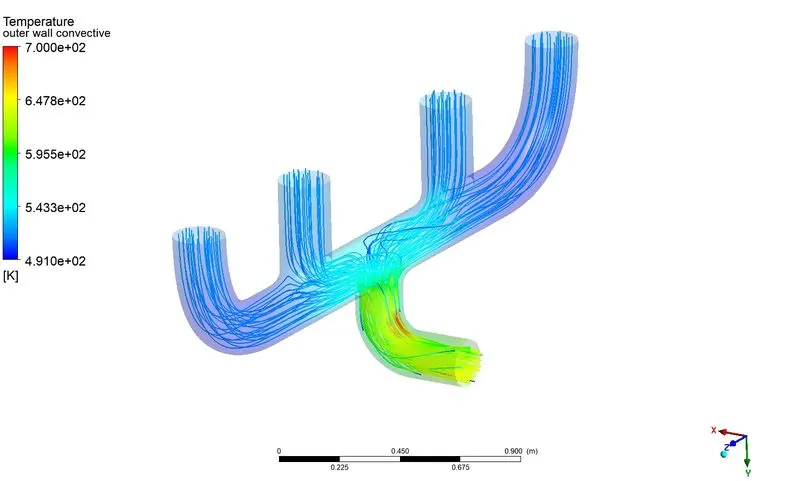
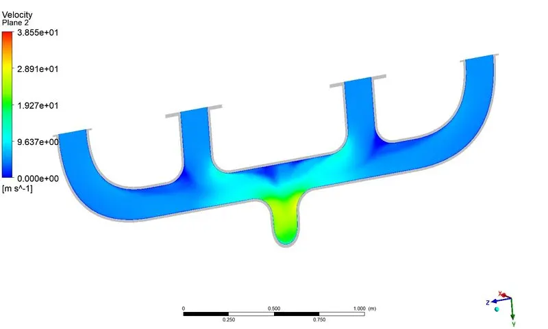
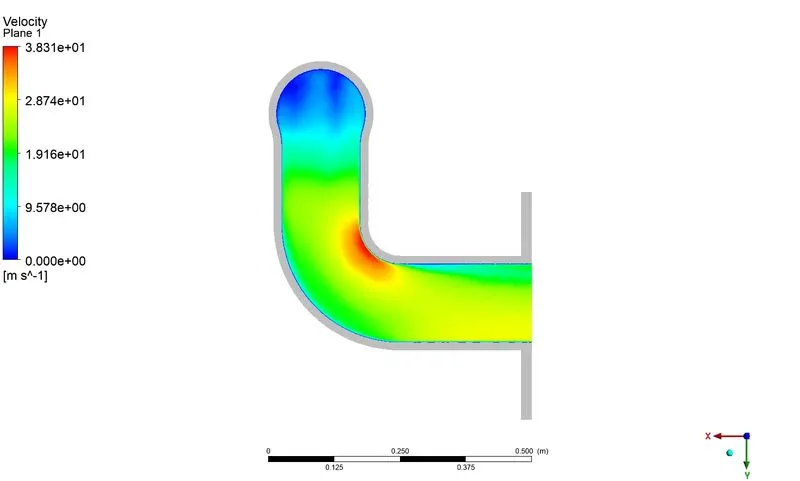
The first figure shows the streamlines inside the pipe and the other two show the velocity contours at different cross-sections to understand the temperature phenomenon.
It is seen from the plots that the velocity is increased when the flow is at the exit. The velocity is maximum for the bend near the exit. This is because of the continuity equation.
The cross-section is almost the same everywhere, hence as per the continuity equation, the mass flow rate needs to be conserved. Here in this problem, the hot fluid is entering the pipe from 4 inlets and it exits one inlet at a time. Therefore in order to match up the incoming flow rate, the flow has to increase the flow velocity. That’s why the velocity is maximum at the bend.
If the velocity is increasing, the Reynolds number increases, and eventually the temperature will increase. Hence more heat transfer near the exit.
- Surface heat transfer coefficient
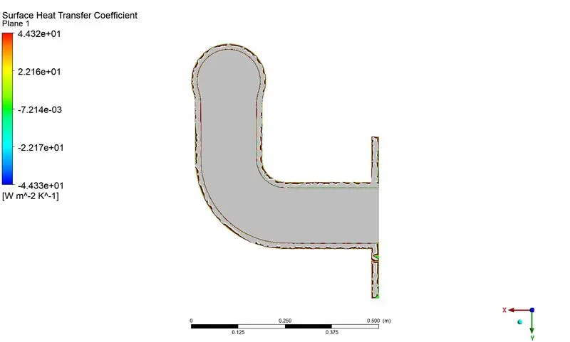
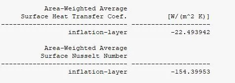
Area weighted average values of surface heat transfer coefficient and Nusselt number are found to be 22.494 and 154.4 respectively.
- Maintaining the y+ value according to the turbulent model
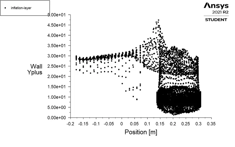
The first figure is when the wall y+=8, which shows that the y+ is varying in between 0 to 45. We can also see that the value is concentrated more in between 2 and 6.
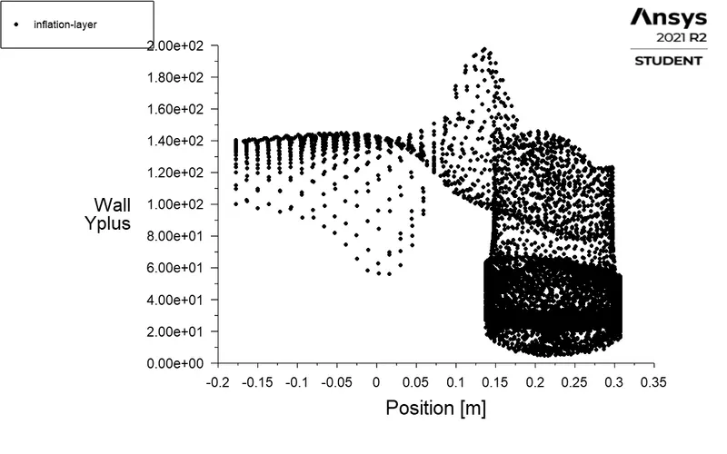
In the second figure, the considered y+=50. It shows that the y+ is varying in between 10 to 200. And the value is more concentrated around 30 to 60.
Since we have taken the k-epsilon model, the y+ needs to be between 30 to 300. Hence, we are opting y+=50 for our analysis.
- Verify heat transfer coefficient prediction from simulation.
From the simulations, we got a surface heat transfer coefficient of 22.49. Let’s cross-check it in an analytical way.
Heat transfer coefficient `h=(N_u k)/L`
For an internal flow,
`N_u=0.023*Re^(0.8)*Pr^(0.4)`
`Pr= (C_p μ)/k`
`C_p=1006`
`k=0.0242 w/(mk)`
Therefore,
`Pr=(1006*1.7894*10^(-5))/0.0242=0.744`
`Nu=0.023*56858.37^0.8*0.744^0.4`
`Nu=130.07`
Therefore,`h=(130.07*0.0242)/0.16611`
`h=18.95`
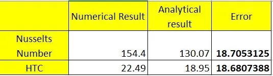
It is observed that there is an error of 18.7% in both HTC and Nusselts numbers.
- Conclusions
- The baseline meshing as well as the refined mesh is showing more or less the same results.
- Choosing the correct inflation layer according to the turbulent model helps to visualize properties near the wall smoothly.
- The heat transfer is more at the bend near the exit because of the conservation of mass flow rate. As the density and cross-section area is constant, flow is increasing the velocity to balance the flow rate which further increases the Reynolds number at the bend and thereby increases the Nusselts number and the heat transfer.