Week 4 - CHT Analysis on Exhaust port
Conjugate Heat Transfer
Conjugate Heat Transfer combines with the combination of heat transfers in solids and heat transfer in fluids. In solids, conduction often dominates whereas in fluids, convection usually dominates. Conjugate heat transfer is observed in many situations. For example, heat sinks are optimized to combine heat transfer by conduction in the heat sink with the convection in the surrounding fluid. The principle of conduction is governed by Fourier's law of heat conduction, whereas convection is influenced by newton's law of cooling.
CHT analysis is beneficial in accurately predicting solid temperature and heat transfer capabilities in engineering devices.
Some applications of CHT
Heat exchangers
A heat exchanger is a system used to transfer heat between two or more fluids. Heat exchangers are used in both cooling and heating processes. The fluids may be separated by a solid wall to prevent mixing or they may be in direct contact.
Aviation
In commercial aircraft, heat exchangers are used to taking heat from the engine's oil systems to heat cold fuel. This improves fuel efficiency, as well as reduces the possibility of water entrapped in the fuel freezing in components.
HVAC
Here air-cooled and liquid-cooled engines, turbochargers, cooling of nuclear reactors, cooling towers, and many more.
Analysis
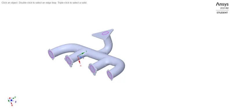
This is the exhaust port we are going to simulate. There are 4 inlets and a single outlet. On simulating we are considering air of temperature 700K, and 5 m/s of velocity, by this we get the value of heat transfer coefficient.
The turbulence model we use is a k-epsilon model.
Case 1
Here we use baseline meshing with no inflation layer and K-epsilon as the turbulence model.
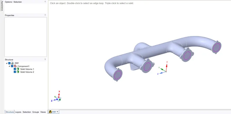
The geometry after preparation and refinement.
Meshing
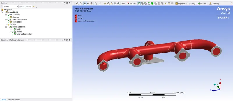
The geometry is defined with 'named selection', as you can see four faces are defined with a name.
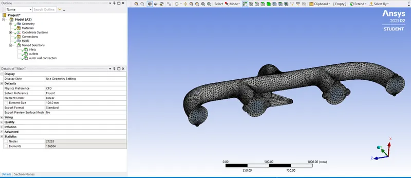
A default meshing is done, with an element size of 100mm. Thereby we get the total number of 136504 cells.
SETUP (FLUENT)
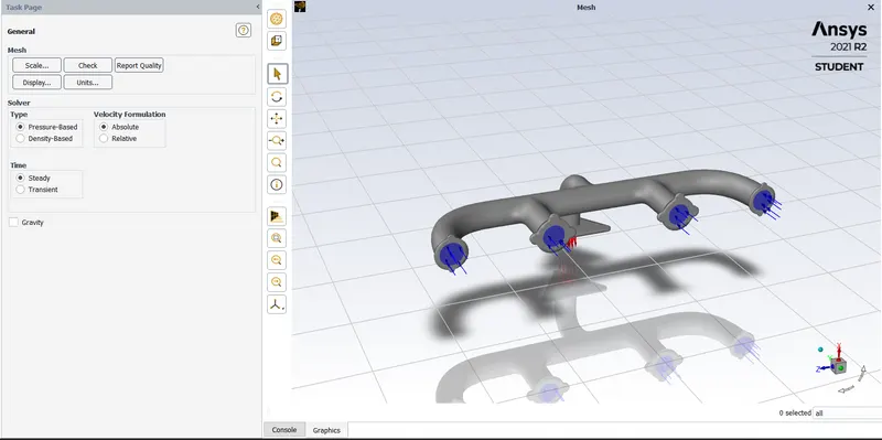
Solver Type - Pressure based
Velocity Formulation - Absolute
Time - Steady
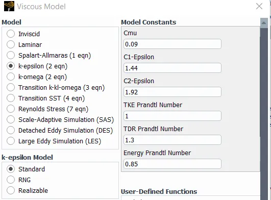
Viscous model - K Epsilon
Material - Aluminium(solid)
Air(Fluid)
Boundary Condition - Inlet Velocity - 5m/s
Temperature - 700K
Outlet Pressure - 0 Pa
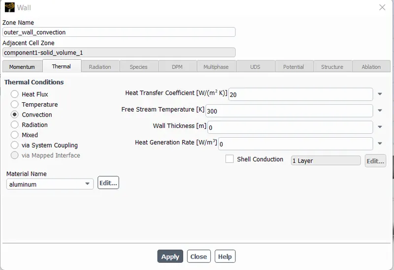
Outer wall convection - Convection
HTC - 20w/m^2 K
Reference Values defined at the inlet.
Area - 0.02167m^2
Length - 0.1661m
Density - 1.225 kg/m^3
Temperature - 700K
Velocity - 5m/s
Results Obtained.
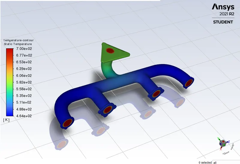
Temperature Contour
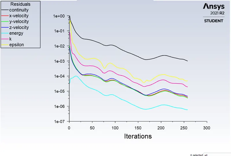
Scaled residuals
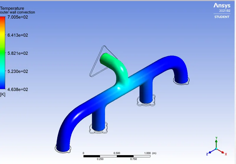
The temperature at outer wall body distribution.
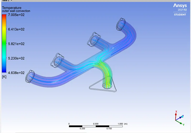
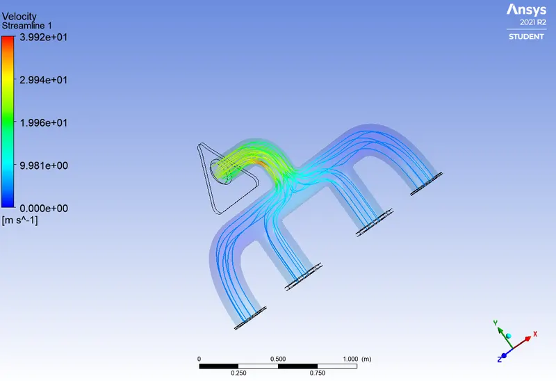
Velocity represented in streamlines
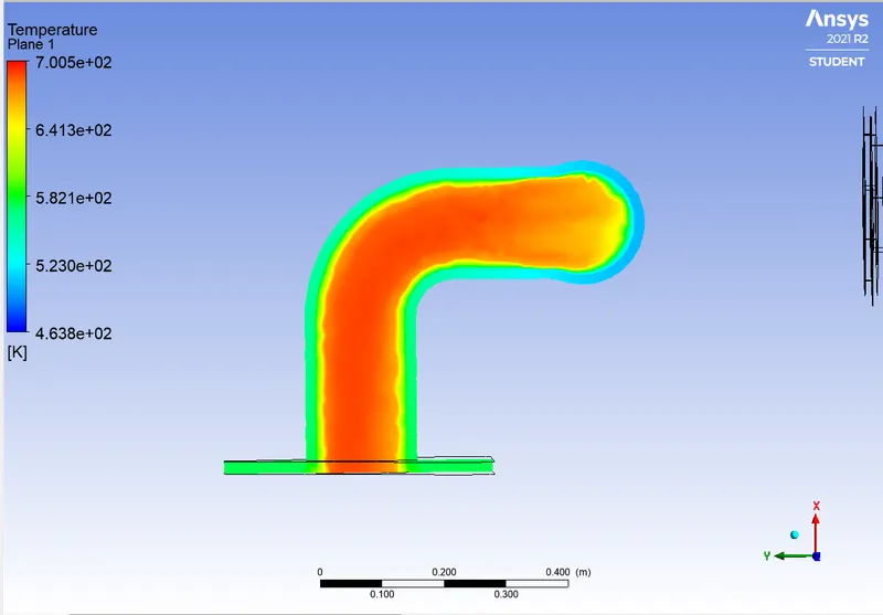
Temperature at the exit pipe (Outlet)
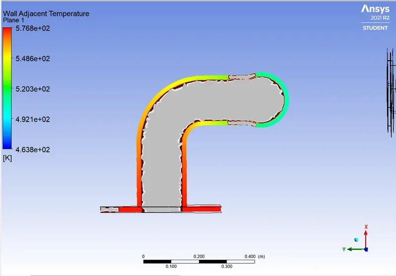
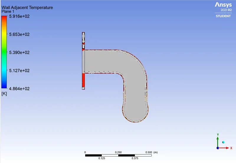
Wall adjacent Temperature at the outlet pipe.
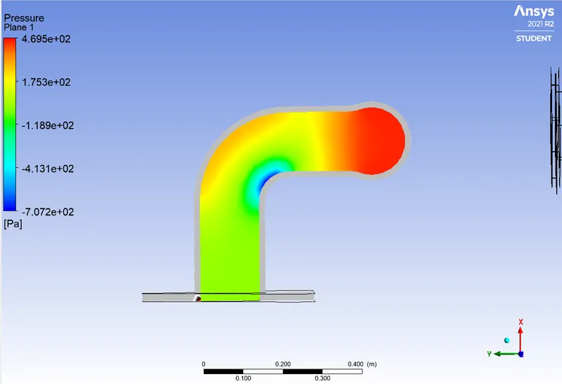
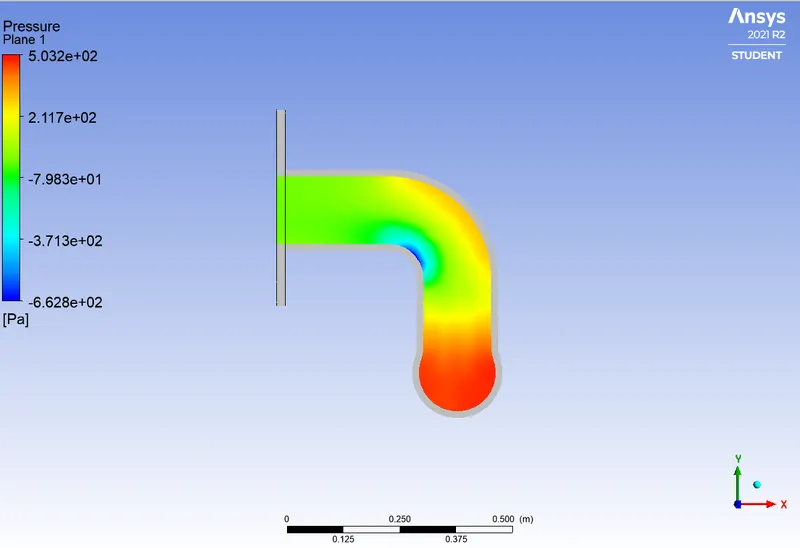
Pressure at the outlet pipe.
CASE 2
Here we are using the k-epsilon Turbulence Model for the simulation. The Y plus value which we used for this simulation is 50.
On using y plus value of 50, we get the First layer Height, Delta S = 2.8mm
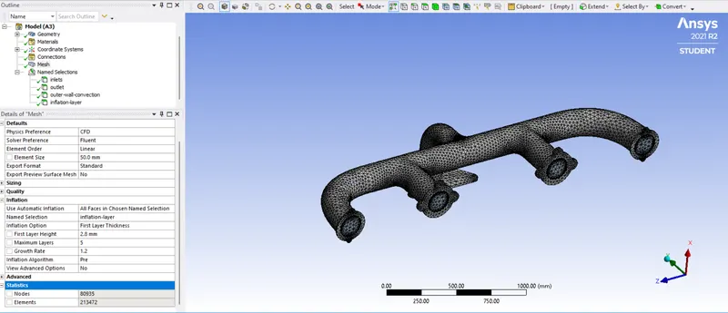
Element sizes are a little more refined, here we use an element size of 50mm.
The Total Number of elements = 213472.
For this simulation, I use the boundary conditions same as the previous case (Case 1)
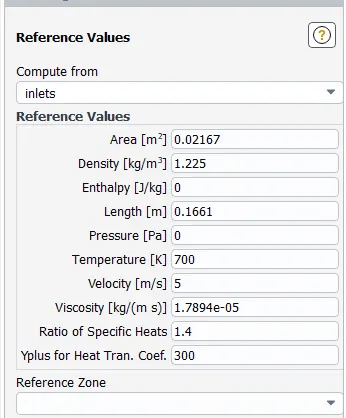
The reference values are given.
After running the iteration 200 times, the results obtained are.
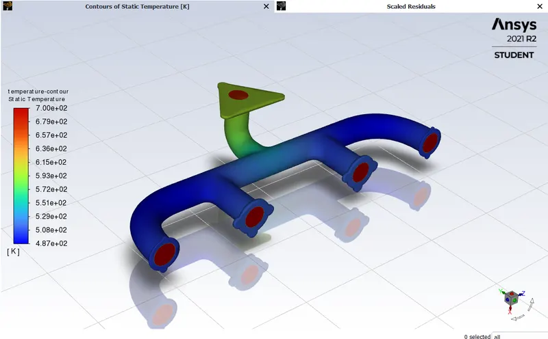
Temperature contour
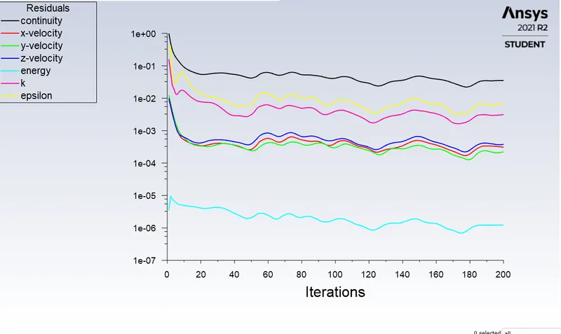
Scaled residuals
After doing the iteration,For finding the Surface Integrals of the results.
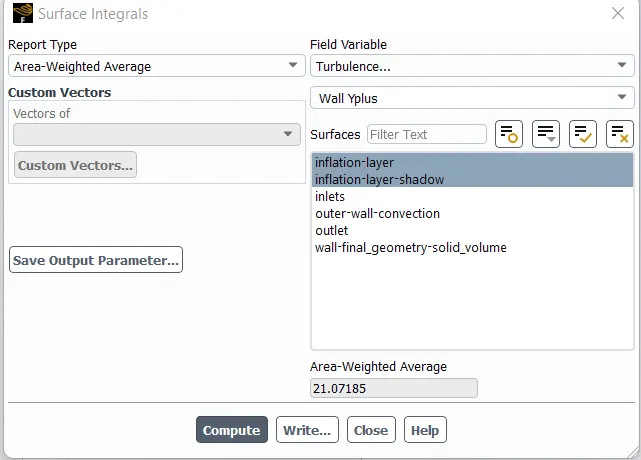
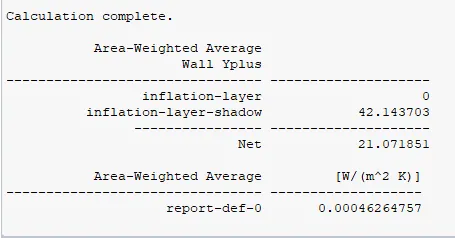
The area-weighted average obtained is 21.07185
On computing the Y-plus, we can see that most of the Y-Plus values are concentrated among the 2.00e+01 and 5.00e+01 regions.
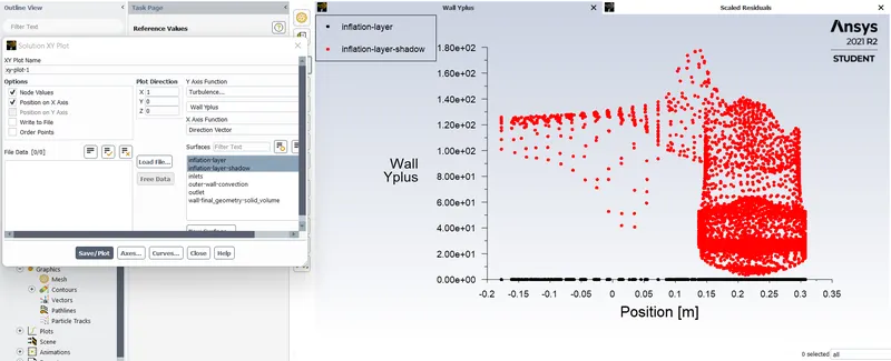
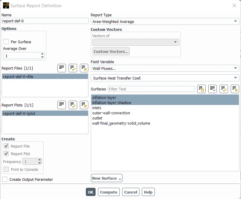
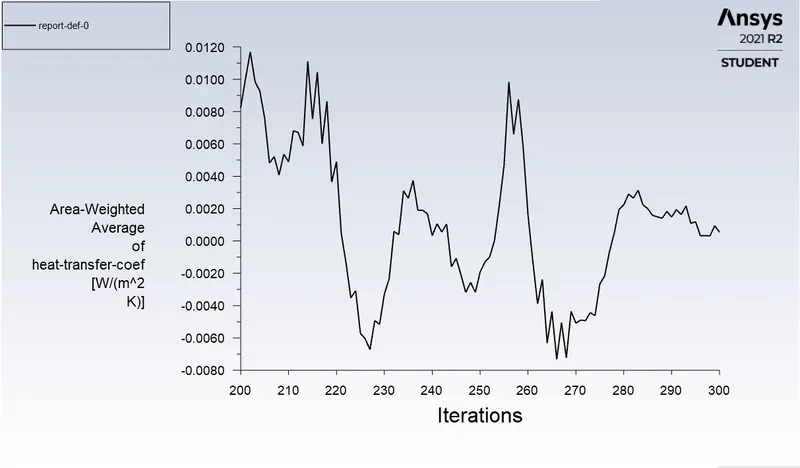
Now, to calculate the report definition on Area-Weighted average
Area Weighted Average Printed on the console.
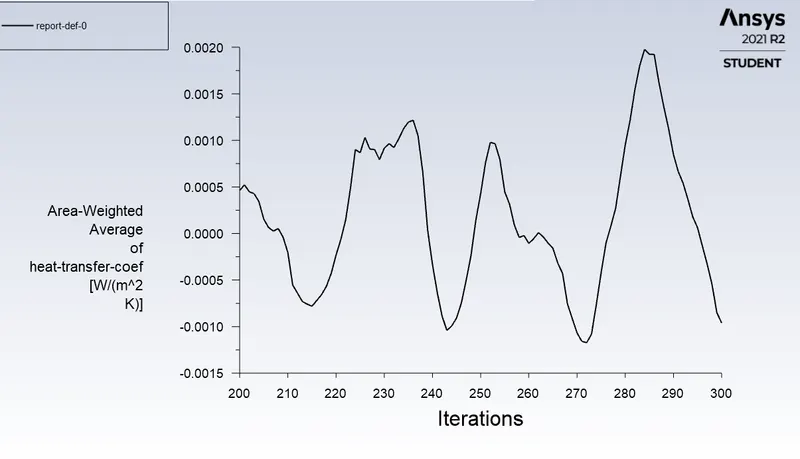
Ansys Post Results.
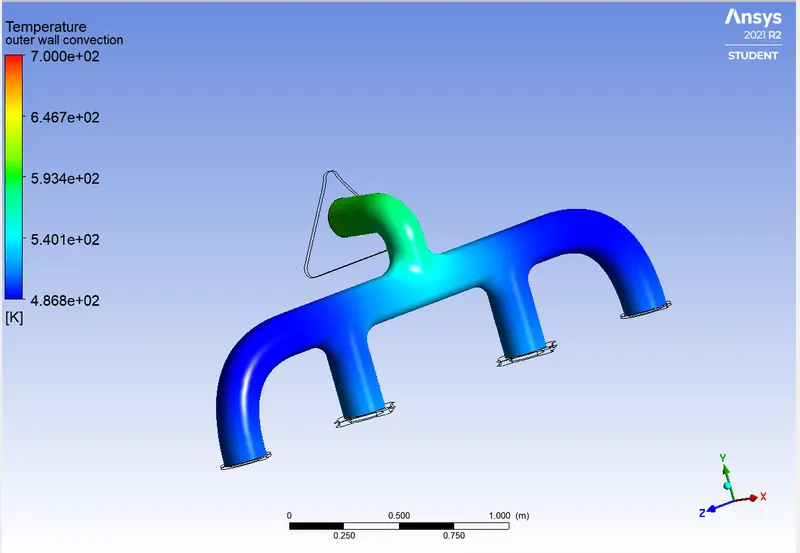
The Temperature contour on the outer body.
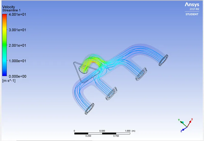
The velocity streamlines on the inner body
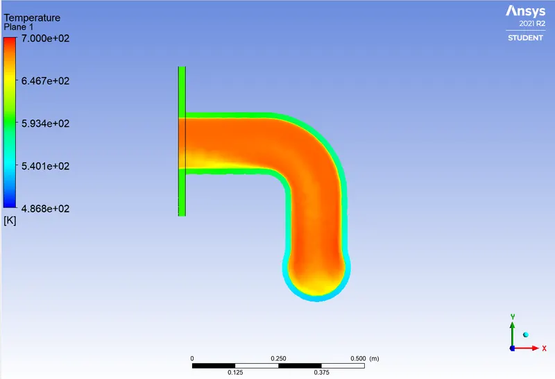
Exit Pipe (outlet) Showing the temperature contour
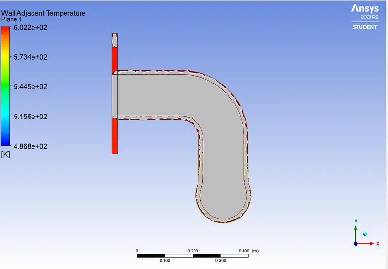
Wall Adjacent Temperature on the outlet pipe.
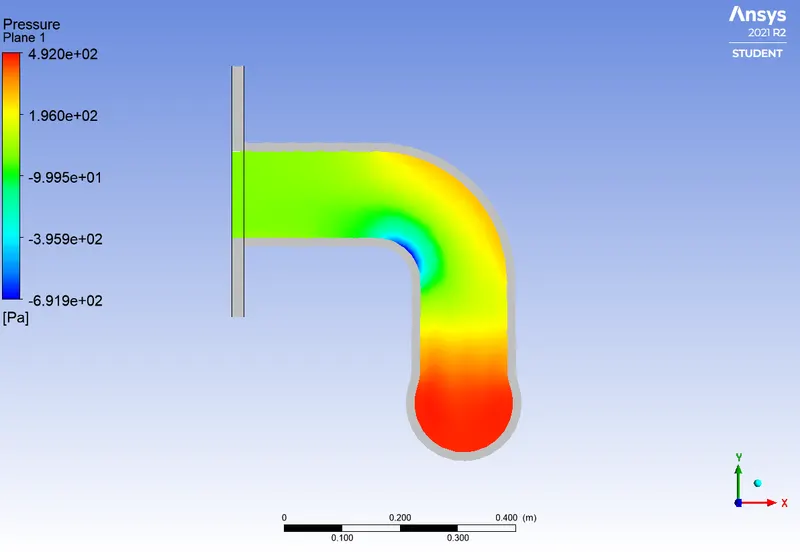
Pressure on the Outlet Pipe.
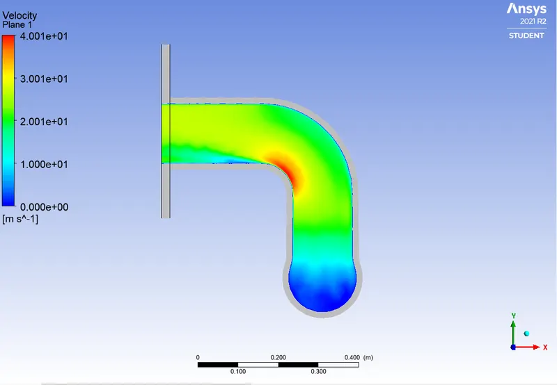
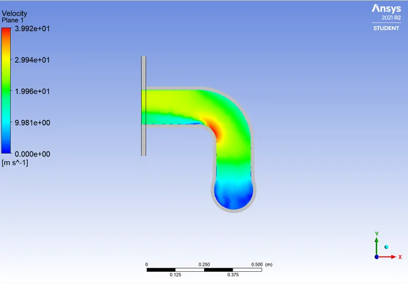
The velocity on the outlet pipe
CASE 3
Here we use K- Omega Turbulence model for the simulation. As we considered using the K-omega Turbulence model, the the Y-Plus value ranges from 0-10. So here i took Y-Plus value = 8. The delta S we got = 0.44mm
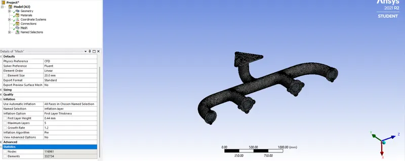
here the element size is a little more refined as compared to the previous one, here the element size given = 20mm.
The first layer height = 0.44mm
and Total number of elements = 332734
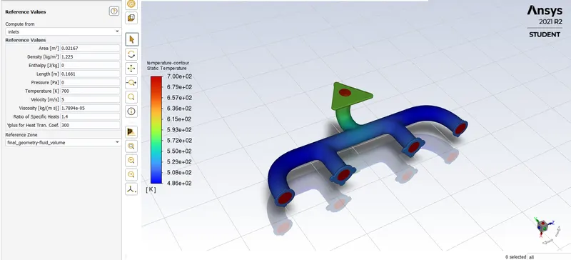
The boundary conditions are the same as in the previous case.
After 200 iterations, the results obtained are.
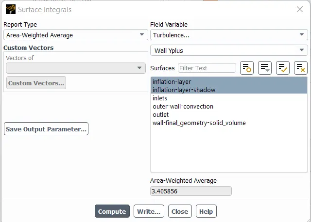
The area-weighted average computed is 3.405856
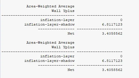
Area-weighted average computed on the console.
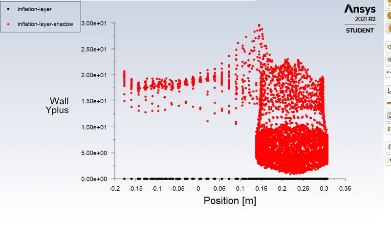
Y-Plus Chart
Post Results
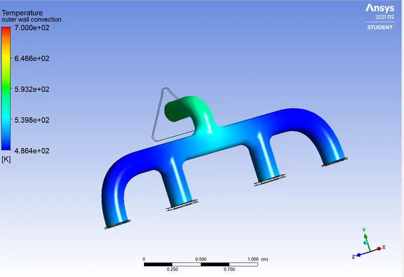
Temperature Contour of the outer body
Internal flow velocity represented with streamed line
The pressure of the Outlet pipe
The velocity of the outlet pipe
Wall Adjacent temperature of the outlet pipe
RESULTS OBTAINED FROM ALL THE CASES
The Conjugate heat transfer (CHT) is in between the solid volume of the exhaust port and the heated fluid volume which is flowing through the exhaust port.
It can be observed from the temperature and velocity contour. The manifold wall attains maximum temperature where the velocity of the fluid flow is highest, this is due to the high Reynolds number intense turbulence ensures efficient heat transfer.
In case 3, K-omega tends to be inherently more consistent because of the efficiency of capturing near-wall effects. A lesser Y+ will produce more approximate results.
HEAT TRANSFER COEFFICIENT
The heat transfer coefficient should be verified with experimental results with the respective flow and thermal conditions.
Analytically heat transfer coefficient can be calculated with the help of the Dittus-Boelter Equation
(when the fluid is heated along with the flow) and (when fluid is cooled along with the flow).
In our case, heated fluid is losing heat to the walls of the exhaust port.
So, Nu = 0.023Re^0.8Pr^0.3 is used to calculate the nusselt number of the respective case.
The heat transfer coefficient is calculated using 'Nu = (hL)/k'
Where,
h = Heat transfer coefficient
L = Hydraulic diameter
k = Thermal Conductivity of the fluid.