Week 4 - CHT Analysis on Exhaust port
Assignment name- CHT (conjugate heat transfer -exhaust port analysis)
Objective-
- perform CHT analysis on an exhaust port and give necessary plot
- How would you verify HTC prediction from the simulation is corrected?
- Factors on which prediction accuracy depends
Why CHT (conjugate heat transfer) is required-
The conjugate heat transfer analysis allows us the simulation of heat transfer between solid and fluid domain by exchanging thermal energy at the inference between them and CHT analysis can be used to generate increased resolution thermal inputs on the stage wetted surface
Where CHT analysis used
- Analysis of heat exchangers,
- analysis of cooling of electronic equipment and many more
conformal meshing-conformal meshing is a technique which can dramatically reduce the memory and time required for analysis of a circuit with diagonal or curved polygon edges. This technique groups together strings of cells following diagonal and curved metal contours to form long subsections along those contour
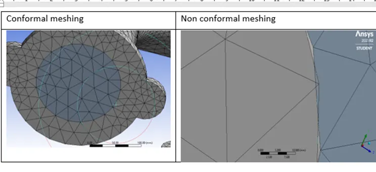
I have performed two simulations for CHT analysis of exhaust port
Case 1- analysis with baseline mesh
Case 2-analysis with finer mesh
Steps involved in the simulation
Geometry
Mesh
Setup
Solution
Results
Case 1-analysis with baseline simulation
Geometry-
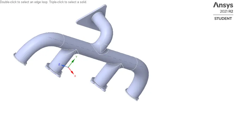
the model is imported to space claim
repair the model with help of extra edge key
extracted fluid volume from the geometry
share the topology for sharing information between solid and fluid
mesh
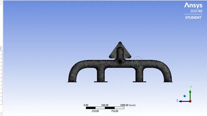
element size-150mm
number of elements-134877
no of nodes-26988
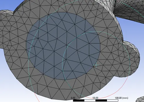
mesh quality
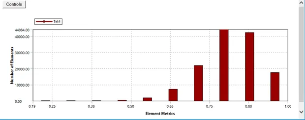
Lowest mesh quality was 19%
setup-
solver type-pressure Based Solver-steady state
model-viscous k-epsilon standard
energy-turn on
boundary condition-
inlet velocity-5m/s
temperature-700k
outlet-pressure outlet
wall convection-heat cooficient-20W/m^2 k
free stream temperature=300k
material properties
fluid-air
solid-aluminium
method-Simple
initialization- Hybrid initialization
solution
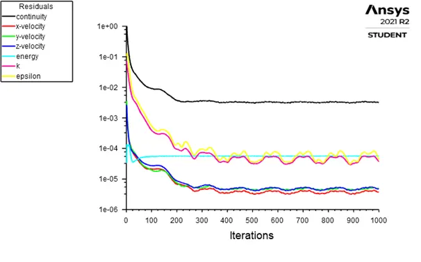
we can easily conclude or assumed that around 750-800 iteration solution is converged. This can be seen by below residual plot as residual is constant and repeated pattern
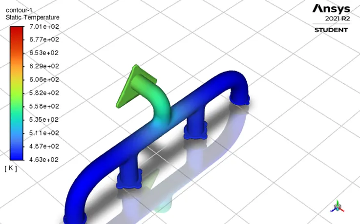
Temperature contour
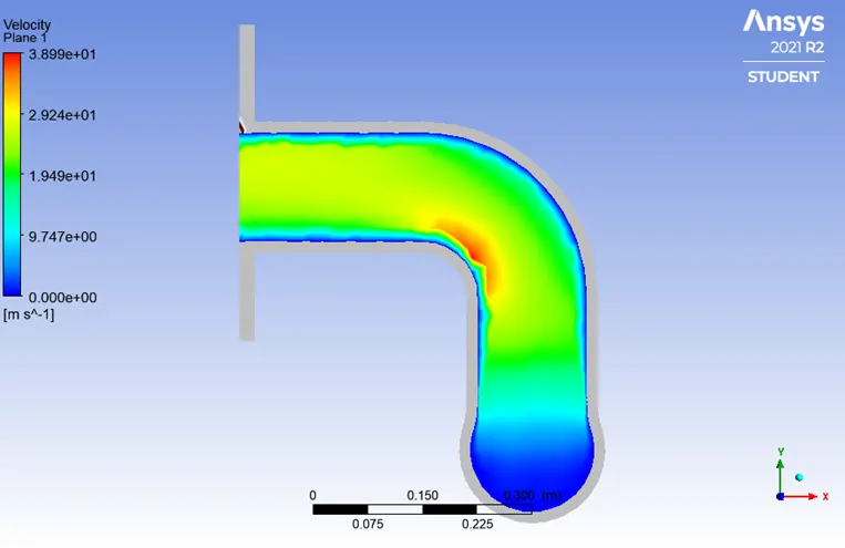
Velocity contour
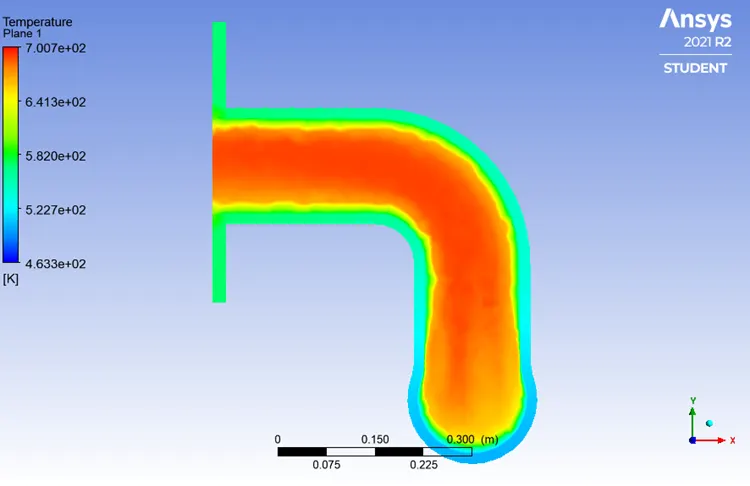
Temperature contour by inserting plane
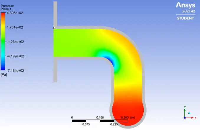
Pressure contour
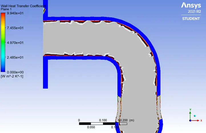
Wall heat transfer coefficient
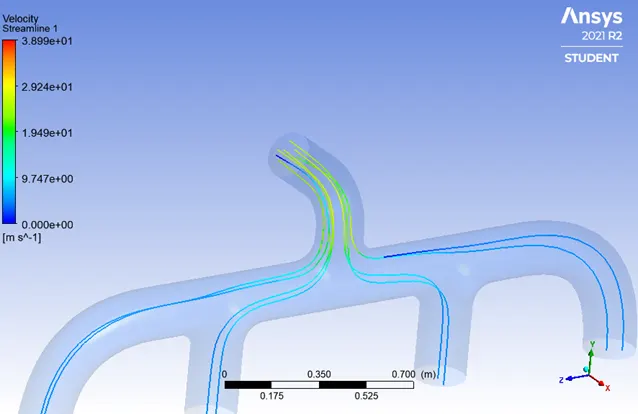
velocity streamline
Case 2-analysis with finer mesh
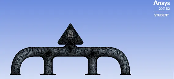
element size-150mm
number of elements-305270
no of nodes-99352
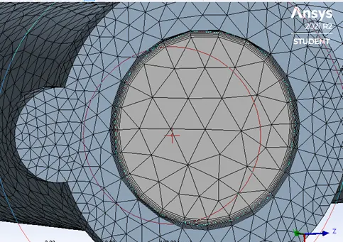
inflation layer total thickness=5mm
number of layer=5
sizing=10mm
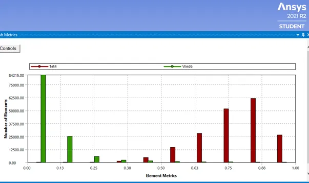
Quality of element
setup-
solver type-pressure Based Solver-steady state
model-viscous k-epsilon standard
energy-turn on
boundary condition-
inlet velocity-5m/s
temperature-700k
outlet-pressure outlet
wall convection-heat cooficient-20W/m^2 k
free stream temperature=300k
material properties
fluid-air
solid-aluminium
method-Simple
initialization- Hybrid initialization
solution
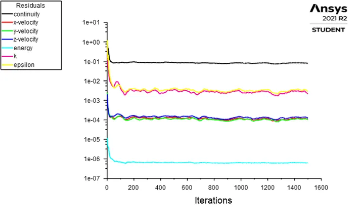
we can easily conclude or assumed that around 1000-2000 iteration solution is converged. This can be seen by below residual plot as residual is constant and repeated pattern
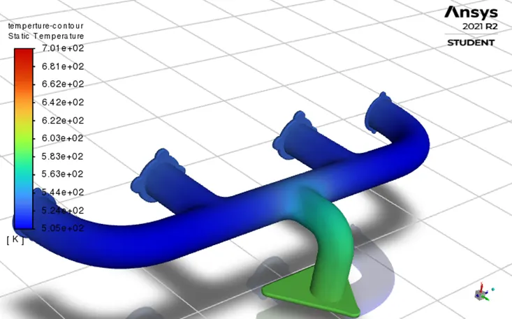
Temperature contour
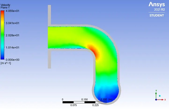
Velocity contour
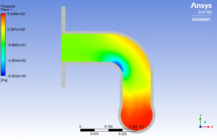
Pressure contour
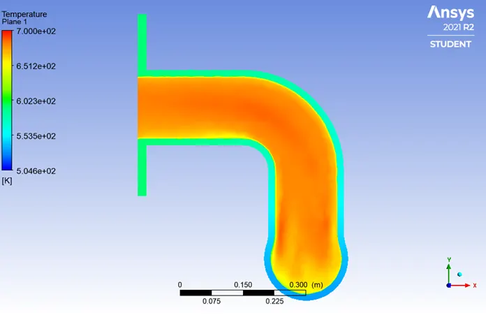
Temperature contour by inserting plane
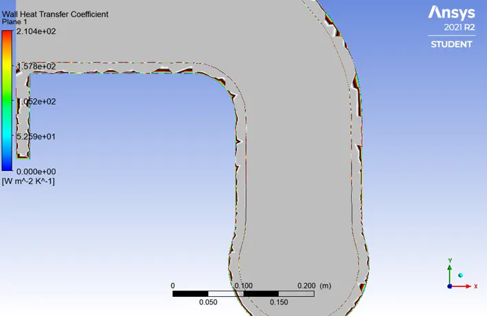
Wall heat transfer coefficient
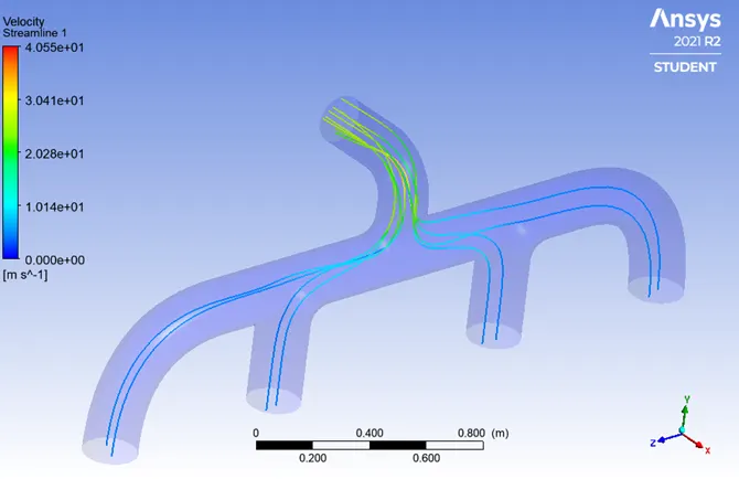
Velocity stream line
how would you verify HTC prediction from the simulation is corrected?
The heat transfer coefficient can be verified by comparing values analytically
We know Nusselt number
Nu=hL/k
h=convective heat transfer coefficient
k= thermal conductivity of fluid
We know Reynold number
Re=(ρVL)/µ
And
Nu=f (Re, Pr)
From above we conclude that Nusselt number is directly proportional to Reynold number and Reynold number is directly proportional velocity
HTC is depending on mass transfer and we know that more the velocity, more rate of mass transfer Then from above information we can easily say that HTC is directly proportional to velocity
And from above statement and contours we say that velocity and HTC is highest at exhaust port i.e., at outlet, so we should say that your results are corrected
Factors on which prediction accuracy depends
- corrected geometry (if any fault in geometry, Repaired the geometry)
- meshing (type of mesh, element size)
- setup of physics (type of viscous model)
Conclusion
The base-line mesh gives accurate results but finer mesh gives much better and more accurate results
Wall heat transfer coefficient is captured smoothly and more accurate in finer meshing
Adding inflation give better results
Conformal mesh also important in meshing