Week 8 - Simulation of a backward facing step in OpenFOAM
Assignment Name- Simulation of a backward facing step in OpenFOAM
Objective
- familiar mesh procedure by using the Open FOAM
- Simulate the flow without using any grading factor (i.e., GF = 1)
- Simulate the flow with grading factor of 0.2. The cells should be finer near the walls (includig the step wall)
Mesh Specifications:
Number of cells along the x-direction (longer dimension) = 200
Number of cells along the y-direction = 10
Use a grading factor- for 1st condition use GF= 1
For second condition Grading factor near all walls should be 0.2
Boundary Condition Specification:
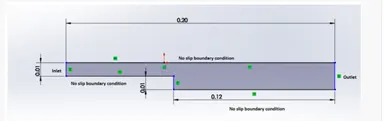
Follow the dimensions to create blocks using Open Foam
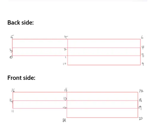
Introduction of Open FOAM:
Open FOAM (for "Open-source Field Operation And Manipulation") is a C++ toolbox for the development of customized numerical solvers, and pre-/post-processing utilities for the solution of continuum mechanics problems, most prominently including Computational Fluid Dynamics (CFD).
Advantages:
- The friendly syntax for partial differential equations
- Fully documented source code
- Unstructured polyhedral grid capabilities
- Automatic parallelization of applications written using OpenFOAM high-level syntax
- Wide range of applications and models ready to use
- Commercial support and training provided by the developers
- No license costs
Disadvantages:
- The development community suffers from fragmentation, giving rise to numerous forked projects.
- Absence of an integrated Graphical User Interface (stand-alone open-source and proprietary options are available).
- The Programmer's guide does not provide sufficient details, making the progress slow if you need to write new applications or add functionality.
- Block:
Simulation: (Steps)
- Open the terminal in the Linux Operating System
- just type 'cd $FOAM_TUTORIALS', and it takes you to the in-built tutorial files of the OpenFOAM software. Type 'ls' (list) to view the contents in the tutorials.
- Type 'cd incompressible'. And then 'ls'. It takes into the incompressible directory file.
- Type 'cd icoFoam', then 'ls'. This step takes into the icoFoam directory file.
- Type 'cd cavity' and 'ls' to list the contents.
- Copy cavity by type 'cp -r cavity/ $FOAM_RUN/'. This command copies the cavity file and pastes directly in the run folder. To check....
- Type 'cd' $FOAM_RUN'. It takes to the run folder which creates automatically by the software and we can see file that we copied. Never run your simulation directly in the tutorial file itself. It may corrupt the entire tutorial file if any mistakes or errors took. To regain those files, we need to uninstall the software and install again which is a long-process.
- Open the files using the change directory 'cd' command.
- In the file you copied, open cavity --> system. Type 'ls' to see the contents.
- There we see blockMeshDict, controlDict, fvschemes and fvslutions are text files which we need to edit the file according to our boundary conditions.
- Type 'gedit blockMeshDict'. Here we give a shape to the problem, applying the mesh grading, allocating the grid numbers to the respective points we assumed and lastly don't forget to save the file.
- Likewise, edit controlDict file also to give limits in words of time, like start time, end time, time interval and deltat.
- While selecting the 'delta t' value, be aware of the courant number. It should be less than one (< 1). Otherwise, the solution may diverge and stopped forcibly by software itself.
- Come back to the cavity file using change directory command 'cd ..' .
- In this file, we need to edit the velocity and pressure files according to the problem. for that, we need to go to '0' file.
- '0' file represents us that the initial conditions of the problem. And these files are inbuilt files. Here at this step, we need to be careful that no-slip conditions, etc.,
After editing the four files, come to the 'cavity' directory. There we need to give a command 'blockMesh' to get mesh structured, and other mesh calculations are done here. After completing it we need to check the mesh that it has any error in it or not. For that, 'checkMesh' command is used.
After completing both the steps, we can confirm that our mesh is stable and good. Now type 'icoFoam' to calculate simulation or problem. Because in the icoFoam file only we copied and pasted the file for run.
After the completion of simulation, type 'paraFoam' for the post-processing.
System directory
1. Block Mesh Directory
/*--------------------------------*- C++ -*----------------------------------*
========= |
\ / F ield | OpenFOAM: The Open Source CFD Toolbox
\ / O peration | Website: https://openfoam.org
\ / A nd | Version: 9
\/ M anipulation |
*---------------------------------------------------------------------------*/
FoamFile
{
format ascii;
class dictionary;
object blockMeshDict;
}
// * * * * * * * * * * * * * * * * * * * * * * * * * * * * * * * * * * * * * //
convertToMeters 0.01;
vertices
(
(0 0 0)
(8 0 0)
(8 0.5 0)
(0 0.5 0)
(8 1 0)
(0 1 0)
(20 1 0)
(20 0.5 0)
(20 0 0)
(20 -1 0)
(8 -1 0)
(0 0 0.1)
(8 0 0.1)
(8 0.5 0.1)
(0 0.5 0.1)
(8 1 0.1)
(0 1 0.1)
(20 1 0.1)
(20 0.5 0.1)
(20 0 0.1)
(20 -1 0.1)
(8 -1 0.1)
);
blocks
(
hex (0 1 2 3 11 12 13 14) (200 10 1) simpleGrading (1 1 1)
hex (3 2 4 5 14 13 15 16) (200 10 1) simpleGrading (1 1 1)
hex (2 7 6 4 13 18 17 15) (200 10 1) simpleGrading (1 1 1)
hex (1 8 7 2 12 19 18 13) (200 10 1) simpleGrading (1 1 1)
hex (10 9 8 1 21 20 19 12) (200 10 1) simpleGrading (1 1 1)
);
edges
(
);
boundary
(
inlet
{
type patch;
faces
(
(0 11 14 3)
(3 14 16 5)
);
}
outlet
{
type patch;
faces
(
(9 8 19 20)
(8 7 18 19)
(7 6 17 18)
);
}
frontAndBack
{
type empty;
faces
(
(0 3 2 1)
(3 5 4 2)
(2 4 6 7)
(1 2 7 8)
(10 1 8 9)
(11 12 13 14)
(14 13 15 16)
(13 18 17 15)
(12 19 18 13)
(21 20 19 12)
);
}
noSlipWalls
{
type wall;
faces
(
(16 15 4 5)
(15 17 6 4)
(10 21 12 1)
(11 0 1 12)
(21 10 9 20)
);
}
);
mergePatchPairs
(
);
// ************************************************************************* //
2.Control directory
/*--------------------------------*- C++ -*----------------------------------*
========= |
\ / F ield | OpenFOAM: The Open Source CFD Toolbox
\ / O peration | Website: https://openfoam.org
\ / A nd | Version: 9
\/ M anipulation |
*---------------------------------------------------------------------------*/
FoamFile
{
format ascii;
class dictionary;
location "system";
object controlDict;
}
// * * * * * * * * * * * * * * * * * * * * * * * * * * * * * * * * * * * * * //
application icoFoam;
startFrom startTime;
startTime 0;
stopAt endTime;
endTime 0.5;
deltaT 1e-05;
writeControl timeStep;
writeInterval 20;
purgeWrite 0;
writeFormat ascii;
writePrecision 6;
writeCompression off;
timeFormat general;
timePrecision 6;
runTimeModifiable true;
// ************************************************************************* //
0 directory (initial condition)
1.P directory
/*--------------------------------*- C++ -*----------------------------------*
========= |
\ / F ield | OpenFOAM: The Open Source CFD Toolbox
\ / O peration | Website: https://openfoam.org
\ / A nd | Version: 9
\/ M anipulation |
*---------------------------------------------------------------------------*/
FoamFile
{
format ascii;
class volScalarField;
object p;
}
// * * * * * * * * * * * * * * * * * * * * * * * * * * * * * * * * * * * * * //
dimensions [0 2 -2 0 0 0 0];
internalField uniform 0;
boundaryField
{
inlet
{
type zeroGradient;
}
outlet
{
type fixedValue;
value uniform 0;
}
noSlipWalls
{
type zeroGradient;
}
frontAndBack
{
type empty;
}
}
// ************************************************************************* //
2.U directory
/*--------------------------------*- C++ -*----------------------------------*
========= |
\ / F ield | OpenFOAM: The Open Source CFD Toolbox
\ / O peration | Website: https://openfoam.org
\ / A nd | Version: 9
\/ M anipulation |
*---------------------------------------------------------------------------*/
FoamFile
{
format ascii;
class volVectorField;
object U;
}
// * * * * * * * * * * * * * * * * * * * * * * * * * * * * * * * * * * * * * //
dimensions [0 1 -1 0 0 0 0];
internalField uniform (0 0 0);
boundaryField
{
inlet
{
type fixedValue;
value uniform (1 0 0);
}
outlet
{
type zeroGradient;
}
noSlipWalls
{
type noSlip;
}
frontAndBack
{
type empty;
}
}
// ************************************************************************* //
change for grading factor
blocks
(
hex (0 1 2 3 11 12 13 14) (200 10 1) simpleGrading (0.2 1.2 1)
hex (3 2 4 5 14 13 15 16) (200 10 1) simpleGrading (0.2 0.2 1)
hex (2 7 6 4 13 18 17 15) (200 10 1) simpleGrading (1.2 0.2 1)
hex (1 8 7 2 12 19 18 13) (200 10 1) simpleGrading (1.2 1.2 1)
hex (10 9 8 1 21 20 19 12) (200 10 1) simpleGrading (1.2 1.2 1)
);
desired output
1.Measure the velocity profile at 0.085 m from the inlet of the geometry for both case studies and compare. You can use the plot over line tool for this.
figure out the right initial conditions
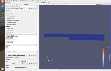
without grading factor (GF=1)
velocity contour
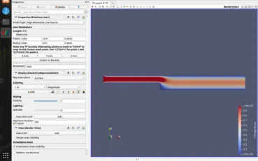
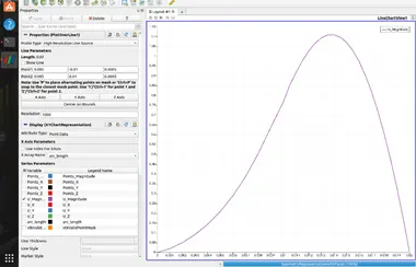
velocity profile at 0.085
with grading factor 0.2
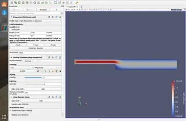
velocity contour
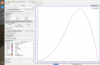
velocity profile at 0.085
how to plot line probe-
- After the simulation runs through, open the case in paraFoam and click apply.
- Then click on the Filters, expand the data analysis group. You will find the plot over line option. If its not present here, use the search option in the filters toolbar and type in “plot over line” to find the option.
- After selecting the plot over line, click apply. Now scroll down the plot over line definition, and input the right values of (x,y,z) coordinate to position the probe, just after the step. After positioning the probe, scroll down further until you find a checklist to select the parameter you want to plot along the line probe.
- Hit apply to get the parameter plotted along the line probe.
- To extract the plot data to an Excel file, click the file option in the toolbar and select the “Export Scene” option. Name the output document and save it.
- Now use the GUI to navigate to the directory where the excel file with the plot data has been save to.
- Note: The line plot can also be done by installing GNUplot and using singleGraph postprocessing command
Conclusion-
Compare the two plots for simple grading and grading factor 0.2 there is negligible difference.
At the grading factor 0.2 Fine mesh is produced and simple grading coarse mesh is produce.
Velocity is maximum at centre of curve minimum at the end because of zero shear stress at the centre
2. why Grading/Growth factor is essential for meshing.
- Specifies the maximum ratio of adjacent mesh edges for transitiong between coarse and fine regions.
- A smaller grading factor produce uniform mesh.