Week 7 - Simulation of a 1D Super-sonic nozzle flow simulation using Macormack Method
Assignment name- MacCormack method
Aim-1-D Supersonic nozzle flow using MacCormack’s method
Objective-
1. Steady-state distribution of primitive variables inside the nozzle
2. Time-wise variation of the primitive variables
3. Variation of Mass flow rate distribution inside the nozzle at different time steps during the time-marching process
4. Comparison of Normalized mass flow rate distributions of both forms
Information regarding MacCormack’s technique- Maccormacks technique is a variant of the Lax-Wendorff approach but its must simpler in its application. Maccormacks technique is also explicit finite differencing technique like Lax-Wendorff approach which is second order accurate in both space and time. Maccormack technique is student friendly technique and easy for coding and understanding the program. And more importantly result obtain form maccormacks technique is satisfactory for many fluids flow application and here we used predictor step and corrected step for getting a result for both conservation and non-conservation form. In maccormack method we used forward differencing for predictor steps and backward differencing for corrector steps
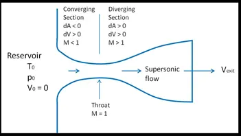
A nozzle for a supersonic flow must increase in area in the flow direction, and a diffuser must decrease in area, opposite to a nozzle and diffuser for a subsonic flow. So, for a supersonic flow to develop from a reservoir where the velocity is zero, the subsonic flow must first accelerate through a converging area to a throat, followed by continued acceleration through an enlarging area.
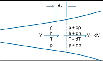
Equations for conservation form and coding hints
In conservation approach we consider or discretise solution in three parts are solution vector, flex vector and source vector for simplification point of view
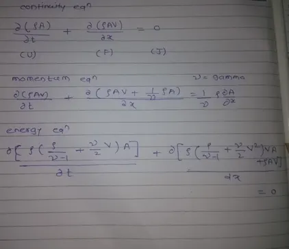
Consider u for solution vector, f for flex vector and J for source vector
Flux term
F1=U2;
F2=(U2.^2./U1)+((gamma-1)/gamma)*(U3-(gamma*U2.^2)./(2*U1));
F3=(gamma*U2.*U3./U1)-(gamma*(gamma-1)/2)*(U2.^3./U1.^2);
Source term
J1=0
J2=(1/gamma)*rho*temp.*(da/dx);
J3=0
Solution vector
U1=rho.*a;
U2=2*U2-U2;
U3=U1*((temp/(gamma-1))+((gamma/2)*V.^2));
dU1/dt= -dF1/dx
dU2/dt= -dF2/dx + J2
dU2/dt= -dF3/dx
boundary condition for conservative form
inlet boundary condition
U1(1)=rho(1).*a(1);
U2(1)=2*U2(2)-U2(3);
U3(1)=U1(1)*((temp(1)/(gamma-1))+((gamma/2)*V(1).^2));
Outlet boundary condition
U1(n)=2*U1(n-1)-U1(n-2);
U2(n)=2*U2(n-1)-U2(n-2);
U3(n)=2*U3(n-1)-U3(n-2);
Note: used forward differencing for predictor step and backward differencing for corrector step
For non-conservative form and coding hint
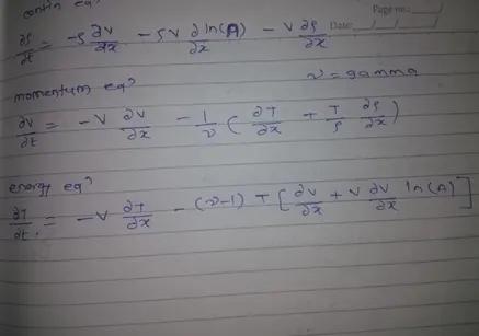
We can’t use here source vector, solution vector and flex term.
While expanding this I insert my code for predictor step and simply we copy this code for corrector step only difference is used backward differencing scheme for corrector steps keep in mind
dVdx=(V(j+1)-V(j))/dx;
drhodx=(rho(j+1)-rho(j))/dx;
dtempdx=(temp(j+1)-temp(j))/dx;
dlogadx=(log(a(j+1))-log(a(j)))/dx;
continuity equation
drhodt_p(j)=-rho(j)*dVdx -rho(j)*V(j)*dlogadx-V(j)*drhodx;
momentum equation
dVdt_p(j)=-V(j)*dVdx-(1/gamma)*(dtempdx+(temp(j)/rho(j))*drhodx);
energy equation
dtdt_p(j)=-V(j)*dtempdx-(gamma-1)*temp(j)*(dVdx+V(j)*dlogadx);
boundary condition for non-conservative form
inlet boundary condition
rho(1)=(1);
temp(1)=(1);
V(1)=2*V(2)-V(3);
Outlet BC conditions
rho(n)=2*rho(n-1)-rho(n-2);
temp(n)=2*temp(n-1)-temp(n-2);
V(n)=2*V(n-1)-V(n-2);
Note: for finding throat position or location we used formula (n+1)/2 where n is number of nodes
Note: while taking energy equation please take precaution while selecting the variables for time and temperature
Function code for conservative form
function[m_c,M_c,V_c,temp_c,p_c,rho_c,rho_th_c,temp_th_c,p_th_c,M_th_c]=conservative(x,dx,n,nt,C,a,gamma,n_th)
%density and temperature for conservative form
for i=1:length(x)
if x(i)>= 0 && x(i)<= 0.5
rho_c(i)=1;
temp_c(i)=1;
else if x(i)>= 0.5 && x(i)<= 1.5
rho_c(i)=1-0.366*(x(i)-0.5);
temp_c(i)=1-0.167*(x(i)-0.5);
else if x(i)>=1.5 && x(i)<= 3.5
rho_c(i)=0.634-0.3879*(x(i)-1.5);
temp_c(i)=0.833-0.3507*(x(i)-1.5);
end
end
end
end
% initializing velocity and pressure
V_c=0.59./(rho_c.*a);
p_c=rho_c.*temp_c;
%initializing the solution vectors
U1=rho_c.*a;
U2=rho_c.*a.*V_c;
U3=rho_c.*a.*((temp_c./(gamma-1))+(gamma/2)*V_c.^2);
% outer time loop
for k=1:nt
% updating old solution vectors
U1_old=U1;
U2_old=U2;
U3_old=U3;
%time steps for conservative form
dt=min(abs((C*dx)./(sqrt(temp_c)+V_c)));
%defining flux vectors
F1=U2;
F2=(U2.^2./U1)+((gamma-1)/gamma)*(U3-(gamma*U2.^2)./(2*U1));
F3=(gamma*U2.*U3./U1)-(gamma*(gamma-1)/2)*(U2.^3./U1.^2);
%Maccormacks method
%predictor step (forward differencing)
for j=2:n-1
J2(j)=(1/gamma).*rho_c(j).*temp_c(j).*((a(j+1)-a(j))/dx);
%predictor step
dU1dt_p(j)=-(F1(j+1)-F1(j))/dx;
dU2dt_p(j)=-((F2(j+1)-F2(j))/dx)+J2(j);
dU3dt_p(j)=-(F3(j+1)-F3(j))/dx;
%updating the new values of solution vectors
U1(j)=U1(j)+dU1dt_p(j)*dt;
U2(j)=U2(j)+dU2dt_p(j)*dt;
U3(j)=U3(j)+dU3dt_p(j)*dt;
end
%update the primitive variables and flux vectors
rho_c=U1./a;
V_c=U2./U1;
temp_c=(gamma-1)*(U3./U1- (gamma/2)*V_c.^2);
p_c=rho_c.*temp_c;
F1=U2;
F2=(U2.^2./U1)+((gamma-1)/gamma)*(U3-(gamma*U2.^2)./(2*U1));
F3=(gamma*U2.*U3./U1)-(gamma*(gamma-1)/2)*(U2.^3./U1.^2);
%move towards corrector step(backward differencing scheme)
for j=2:n-1
J2(j)=(1/gamma)*rho_c(j).*temp_c(j).*((a(j)-a(j-1))/dx);
dU1dt_c(j)=-(F1(j)-F1(j-1))/dx;
dU2dt_c(j)=-((F2(j)-F2(j-1))/dx)+J2(j);
dU3dt_c(j)=-(F3(j)-F3(j-1))/dx;
end
%updating the values of solution vectors
%averaging both predictor and corrector steps for get actual answer
%or appropeiate answer
dU1dt=0.5*(dU1dt_p+dU1dt_c);
dU2dt=0.5*(dU2dt_p+dU2dt_c);
dU3dt=0.5*(dU3dt_p+dU3dt_c);
% calculating the new solution vectors
for i=2:n-1
U1(i)=U1_old(i)+dU1dt(i)*dt;
U2(i)=U2_old(i)+dU2dt(i)*dt;
U3(i)=U3_old(i)+dU3dt(i)*dt;
end
%applying BC
%inlet BC
U1(1)=rho_c(1).*a(1);
U2(1)=2*U2(2)-U2(3);
U3(1)=U1(1)*((temp_c(1)/(gamma-1))+((gamma/2)*V_c(1).^2));
% Outlet BC
U1(n)=2*U1(n-1)-U1(n-2);
U2(n)=2*U2(n-1)-U2(n-2);
U3(n)=2*U3(n-1)-U3(n-2);
% updation of the primitive variables
rho_c=U1./a;
V_c=U2./U1;
temp_c=(gamma-1)*(U3./U1-(gamma/2)*V_c.^2);
%defining values for Mach number ,flow rate and pressure
M_c=V_c./sqrt(temp_c);
m_c =rho_c.*a.*V_c;
p_c=rho_c.*temp_c;
%calculating the values of specific quantities at throat position
M_th_c(k)=M_c(n_th);
rho_th_c(k)=rho_c(n_th);
p_th_c(k)=p_c(n_th);
temp_th_c(k)=temp_c(n_th);
% comparison mass flow rates at different timesteps
figure(1);
hold on;
grid on;
if k== 1
plot(x,m_c,'b')
else if k== 100
plot(x,m_c,'g')
else if k== 200
plot(x,m_c,'k')
else if k== 700
plot(x,m_c,'k')
end
end
end
end
end
title('comparison of mass flow rates at different time steps- Conservative form');
legend('1','100','200','700');
xlabel('X');
ylabel('mass flow rate');
axis([0 3 0.5 0.7]);
end
Function code for non-conservative form
function[m,M,V,temp,p,rho,rho_th,temp_th,p_th,M_th]=non_conservative(x,dx,n,nt,C,a,gamma,n_th);
%%non conservative governing equations
%primitive variables
rho=1-0.3146*x;
temp=1-0.2314*x;
V=(0.1+1.09*x).*temp.^0.5;
% outer time loop
for k=1:nt
% update primitive varibles
rho_old=rho;
temp_old=temp;
V_old=V;
%time steps for non conservative form
dt=min(abs((C.*dx)./(sqrt(temp)+V)));
%predictor method (forward differencing scheme)
for j=2:n-1
dVdx=(V(j+1)-V(j))/dx;
drhodx=(rho(j+1)-rho(j))/dx;
dtempdx=(temp(j+1)-temp(j))/dx;
dlogadx=(log(a(j+1))-log(a(j)))/dx;
%continuity equation
drhodt_p(j)=-rho(j)*dVdx -rho(j)*V(j)*dlogadx-V(j)*drhodx;
%mometum equation
dVdt_p(j)=-V(j)*dVdx-(1/gamma)*(dtempdx+(temp(j)/rho(j))*drhodx);
%energy equation
dtdt_p(j)=-V(j)*dtempdx-(gamma-1)*temp(j)*(dVdx+V(j)*dlogadx);
%solution update
rho(j)=rho(j)+drhodt_p(j)*dt;
V(j)=V(j)+dVdt_p(j)*dt;
temp(j)=temp(j)+dtdt_p(j)*dt;
end
%now move towards corrector step (backward differencing schme)
for j=2:n-1
dVdx=(V(j)-V(j-1))/dx;
drhodx=(rho(j)-rho(j-1))/dx;
dtempdx=(temp(j)-temp(j-1))/dx;
dlogadx= (log(a(j))-log(a(j-1)))/dx;
%continuity equation
drhodt_c(j)=-rho(j)*dVdx-rho(j)*V(j)*dlogadx-V(j)*drhodx;
% momentum equation
dVdt_c(j)=-V(j)*dVdx-(1/gamma)*(dtempdx+(temp(j)/rho(j))*drhodx);
%energy equation
dtdt_c(j)=-V(j)*dtempdx-(gamma-1)*temp(j)*(dVdx+V(j)*dlogadx);
end
%averaging for both predictor and corrector steps
dVdt=0.5*(dVdt_p+dVdt_c);
drhodt=0.5*(drhodt_p+drhodt_c);
dtdt=0.5*(dtdt_p+dtdt_c);
% calculating the updated solution
for i=2:n-1
V(i)=V_old(i)+dVdt(i)*dt;
rho(i)=rho_old(i)+drhodt(i)*dt;
temp(i)=temp_old(i)+dtdt(i)*dt;
end
%applying BC
%inlet BC conditions
rho(1)=(1);
temp(1)=(1);
V(1)=2*V(2)-V(3);
% Outlet BC conditions
rho(n)=2*rho(n-1)-rho(n-2);
temp(n)=2*temp(n-1)-temp(n-2);
V(n)=2*V(n-1)-V(n-2);
%defining values for Mach number,flow rate and pressure
M=V./sqrt(temp);
m =rho.*a.*V;
p=rho.*temp;
%calculating the values of quantities at throat
M_th(k)=M(n_th);
rho_th(k)=rho(n_th);
p_th(k)=p(n_th);
temp_th(k)=temp(n_th);
% comparison of mass flow rates at different timesteps
figure(2);
grid on
hold on
if k==50
plot(x,m,'g')
else if k== 100
plot(x,m,'r')
else if k == 150
plot(x,m,'b')
else if k==200
plot(x,m,'k')
else if k==700
plot(x,m,'m')
end
end
end
end
end
end
title('comparison of mass flow rates at different time steps- Non Conservative form');
legend('50','100','150','200','700');
xlabel('X');
ylabel('mass flow rate');
axis([0 3 0 2.5]);
end
Main MATLAB Code
%%maccormacks methods clarification
clear all
close all
clc
L=3;
n=31;
x=linspace(0,L,n);
dx=x(2)-x(1);
gamma=1.4;
C=0.5;
nt=1000;
%throat location
n_th=(n+1)/2;
%area
a=1+2.2*(x-1.5).^2;
% constact mass flow rate across the nozzle is the exact solution
m_ex=linspace(0.579,0.579,n);
% solution by conservative form
tic
[m_c,M_c,V_c,temp_c,p_c,rho_c,rho_th_c,temp_th_c,p_th_c,M_th_c]=conservative(x,dx,n,nt,C,a,gamma,n_th)
simulation_time_c=toc;
fprintf('The computation time for conservative form : %f',simulation_time_c);
% solution by non-conservative form
tic
[m,M,V,temp,p,rho,rho_th,temp_th,p_th,M_th]=non_conservative(x,dx,n,nt,C,a,gamma,n_th);
simulation_time=toc;
fprintf('The computation time for the non-conservative form is %f',simulation_time);
% Variation of density,temperature,pressure and Mach number against time
figure(3)
subplot(4,1,1)
plot(M_th_c,'b');
hold on
plot(M_th,'r');
hold off
grid on
ylabel('Mach number')
legend('conservative form','non conservative form')
subplot(4,1,2)
plot(temp_th_c,'b');
hold on
plot(temp_th,'r');
hold off
grid on
ylabel('temperature')
legend('conservative form','non conservative form')
subplot(4,1,3)
plot(p_th_c,'b');
hold on
plot(p_th,'r');
hold off
grid on
ylabel('pressure')
legend('conservative form','non conservative form')
subplot(4,1,4)
plot(rho_th_c,'b');
hold on
plot(rho_th,'r');
hold off
grid on
ylabel('density')
legend('conservative form','non conservative form')
%variation along x
figure(4)
subplot(4,1,1)
plot(x,M_c,'b')
hold on
plot(x,M,'*k')
hold off
grid on
legend('conservative form','non conservative form')
title(' varation along x')
xlabel('x')
ylabel('mach number')
subplot(4,1,2)
plot(x,temp_c,'b')
hold on
plot(x,temp,'*k')
hold off
grid on
legend('conservative form','non conservative form')
title(' varation along x')
xlabel('x')
ylabel('temperature')
subplot(4,1,3)
plot(x,p_c,'b')
hold on
plot(x,p,'*k')
hold off
grid on
legend('conservative form','non conservative form')
title(' varation along x')
xlabel('x')
ylabel('pressure')
subplot(4,1,4)
plot(x,rho_c,'b')
hold on
plot(x,rho,'*k')
hold off
grid on
legend('conservative form','non conservative form')
title(' varation along x')
xlabel('x')
ylabel('density')
%%%%compare mass flow rate
figure(5)
plot(x,m_c,'r')
hold on
plot(x,m,'b')
hold on
plot(x,m_ex,'g')
hold off
grid on
legend('conservative form','non conservative form','exact solution')
title('comparision with exact sloution')
Results and outputs
At n=31
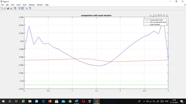
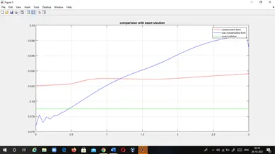
From above plot we can easily conclude that conservative form gives a better result than non-conservative form. The mass flow rate value of conservative from is closer than exact or analytical solution . and we also conclude that conservative from results are more accuracy than non-conservative form
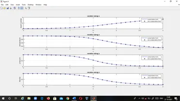
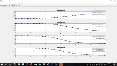
Variations for all quantities along with length is same in both forms. Obliviously Mach number increase form convergent to divergent and graph gives same results. And form plot 2,3,4 we conclude that pressure, temperature and density decrease
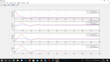
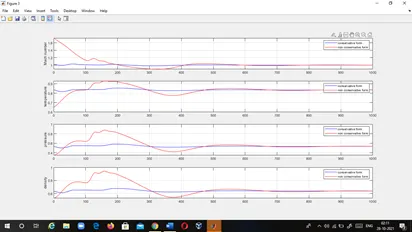
There is slightly lesser variation in non-conservative initially and then as time steps goes on increases it will be steady state and both forms reach steady state. Form this graph we conclude that non-conservative form as closer values of primitive variables to the exact solution
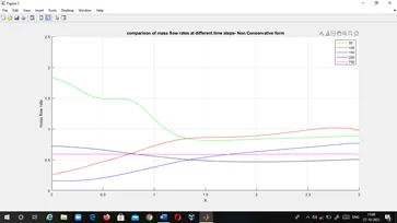
First few steps flow is oscillated or fluctuating When solution become steady state changes with solution is negligible. After these changes is completely resolve we will get your final results. The oscillation shows initially because of unsteady compression and expansion waves
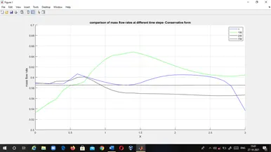
When solution become steady state changes with solution is negligible. After these changes is completely resolve we will get your final results. The oscillation shows initially because of unsteady compression and expansion waves
At n=61
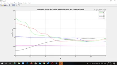
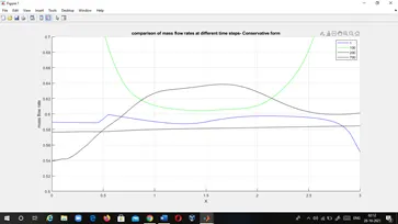
Note- At n=61 plots only for compare with n=31 and study purpose
Simulation time
At n=31
For conservative form=4.3161
For non-conservative form=3.9442
At n=61
For conservative form=4.4099
For non-conservative form=4.1097