Week 5.1 - Mid term project - Solving the steady and unsteady 2D heat conduction problem
Aim-Solving steady and Unsteady 2D heat conduction Problem
Given data-
Top Boundary = 600 K
Bottom Boundary = 900 K
Left Boundary = 400 K
Right Boundary = 800 K
You will implement the following methods for solving implicit equations.
- Jacobi
- Gauss-seidel
- Successive over-relaxation
Your absolute error criteria is 1e-4 (tolerance)
Basic information for code-
1.steady state-
We have equation for steady State equation of 2D heat conduction
(d^2T/dx^2) +(d^2T/dy^2) =0
Consider a square plate for this analysis.
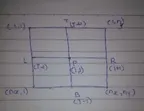
Further simplification we get
Tp=1/k[(TL+TR)/dx^2]+1/k[(TB+TT)/dy^2]
K=2*(dx^2+dy^2)/(dx^2*dy^2)
dx=dy
At the end we get the formula
T(i,j)=0.25*[T(i-1,j)+T(i+1,j)+T(i,j-1)+T(i,j+1)];
Used above formula for
Jacobi iteration scheme
Gauss seidel iteration scheme
And successive over relaxation iteration scheme
We used
T(i,j)=(1-w)*T +w*0.25*[T(i-1,j)+T(i+1,j)+T(i,j-1)+T(i,j+1)];
Consider omega=w=1.2-1.4 because of stability purpose
2.Unsteady State
We have equation for steady State equation of 2D heat conduction
(dT/dt) + alpha(d^2T/dx^2) +(d^2T/dy^2) =0
Consider a square plate for this analysis.
Further simplification we get
alpha=1.4;
k1=(alpha*dt)/dx^2;
k2=(alpha*dt)/dy^2;
term1=(1/(1+(2*k1) +(2*k2)));
term2=term1*k1;
term3=term1*k2;
above consideration follow question and then simply we get,
H=term2*(T(i-1,j)+T(i+1,j));
V=term3*(T(i,j-1)+T(i,j+1));
L=term1*T1(i,j);
T(i,j)=L+H+V;
For above equation follow MATLAB Code or below images or hint image given in question
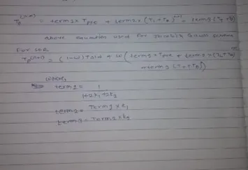
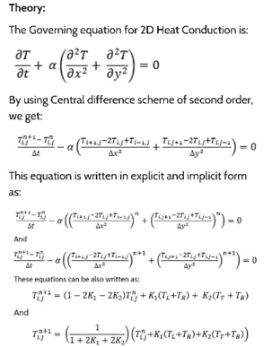
Note-for explicit method do not used iterative solver because all values are known and for implicit method, we should use iterative solver
Some information of steady state and unsteady state-
The main difference between steady state and unsteady state is In steady state the temperature is constant throughout time and unsteady state temperature is changes with time
Some information of Jacobian gauss seidel and Successive Over Relaxation method –
- Jacobian- it gives solution for strictly diagonally dominant system of linear equation and it os slower convergence than gauss seidel and Successive Over Relaxation method
- Gauss seidel- It also known as Liebman method or method of successive displacement and this method give faster convergence than Jacobian Method
- Successive Over Relaxation -SOR is variant of the gauss seidel method for solving a linear system of equations, Resulting in faster convergence
MATLAB CODE
1.Steady state
%%%sloving heat conducttion equation by using steady state method
clear all
close all
clc
%steady state analysis
nx=25;
ny=25;
nx=ny;
l=1;
x=linspace(0,l,nx);
dx=x(2)-x(1);
y=linspace(0,l,ny);
dy=y(2)-y(1);
[XX,YY]=meshgrid(x,y);
%%initial condition
T_left=400;
T_top=600;
T_right=800;
T_bottom=900;
%%%assining array
T=300*ones(nx,ny);
T(:,1)=T_left;
T(:,end)=T_right;
T(1,:)=T_top;
T(end,:)=T_bottom;
%%temperature at nodes
T(1,1)=500;
T(nx,1)=650;
T(1,ny)=700;
T(nx,ny)=850;
%%Given condition and assume initial condition
tol=1e-4;
error=1e9;
%some assumption requried
Told1=T;Told2=T;Told3=T;
T1=T;T2=T;T3=T;
T_initial=T;
itration_slover=3;
w=1.2;
%%%%jacobi itration
if itration_slover==1;
jacobi_iter=1;
tic
while error>tol
for i=2:nx-1
for j=2:ny-1
T1(i,j)=0.25*(Told1(i-1,j)+Told1(i+1,j)+Told1(i,j-1)+Told1(i,j+1));
end
end
error=max(max(abs(Told1-T1)));
Told1=T1;
jacobi_iter=jacobi_iter+1;
end
simulation_time1=toc;
figure(1)
[C,h]=contourf(XX,flip(YY),T1);
xlabel('x')
ylabel('y')
clabel(C,h)
colorbar
colormap(jet)
title_text=sprintf('itreation number=%d',jacobi_iter);
title(title_text)
pause(0.03)
grid on
end
%%GS
if itration_slover==2;
GS_iter=1;
tic
while error>tol
for i=2:nx-1
for j=2:ny-1
T2(i,j)=0.25*(T2(i-1,j)+Told2(i+1,j)+T2(i,j-1)+Told2(i,j+1));
end
end
error=max(max(abs(Told2-T2)));
Told2=T2;
GS_iter=GS_iter+1;
end
simulation_time2=toc;
figure(2)
[C,h]=contourf(XX,flip(YY),T2);
xlabel('x')
ylabel('y')
clabel(C,h)
colorbar
colormap(jet)
title_text=sprintf('itreation number=%d',GS_iter);
title(title_text)
pause(0.03)
grid on
end
%%SOR
if itration_slover==3;
SOR_iter=1;
tic
while error>tol
for i=2:nx-1
for j=2:ny-1
T3(i,j)=(1-w)*Told3(i,j)+(w*0.25*(T3(i-1,j)+Told3(i+1,j)+T3(i,j-1)+Told3(i,j+1)));
end
end
error=max(max(abs(Told3-T3)));
Told3=T3;
SOR_iter=SOR_iter+1;
end
simulation_time3=toc;
figure(3)
[C,h]=contourf(XX,flip(YY),T3);
xlabel('x')
ylabel('y')
clabel(C,h)
colorbar
colormap(jet)
title_text=sprintf('itreation number=%d',SOR_iter);
title(title_text)
pause(0.03)
grid on
end
2.Unsteady
1.Explicit
%%%sloving heat conducttion equation by using Explicit trasient method
%%not used itration slover method we can directly slove this equation using this method
%%%sloving heat conducttion equation by using explicit trasient method
clear all
close all
clc
%explicit transient state analysis
nx=25;
ny=25;
nx=ny;
l=1;
x=linspace(0,l,nx);
dx=x(2)-x(1);
y=linspace(0,l,ny);
dy=y(2)-y(1);
[XX,YY]=meshgrid(x,y);
%%initial condition
T_left=400;
T_top=600;
T_right=800;
T_bottom=900;
%%%assining array
T=300*ones(nx,ny);
T(:,1)=T_left;
T(:,end)=T_right;
T(1,:)=T_top;
T(end,:)=T_bottom;
%%temperature at nodes
T(1,1)=500;
T(nx,1)=650;
T(1,ny)=700;
T(nx,ny)=850;
%%Given condition and assume initial condition
tol=1e-4;
error=1e9;
%some assumption requried
Told=T;
dt=0.1;
t=100;
nt=t/dt;
alpha=1.4;
k1=(alpha*dt)/dx^2;
k2=(alpha*dt)/dy^2;
term1=(1/(1+(2*k1)+(2*k2)));
term2=term1*k1;
term3=term1*k2;
%%%%Calculation
iter=1;
tic
for k=1:nt
for i=2:nx-1
for j=2:ny-1
H=term2*(Told(i-1,j)+Told(i+1,j));
V=term3*(Told(i,j-1)+Told(i,j+1));
L=term1*Told(i,j);
T(i,j)=L+H+V;
end
end
error=max(max(abs(Told-T)));
Told=T;
iter=iter+1;
end
simulation_time1=toc;
figure(1)
[C,h]=contourf(XX,flip(YY),T);
xlabel('x')
ylabel('y')
clabel(C,h)
colorbar
colormap(jet)
title_text=sprintf('itreation number=%d',iter);
title(title_text)
pause(0.03)
grid on
2.Implicit
%%%sloving heat conducttion equation by using implicit trasient method
clear all
close all
clc
%Implicit transient state analysis
nx=25;
ny=25;
nx=ny;
l=1;
x=linspace(0,l,nx);
dx=x(2)-x(1);
y=linspace(0,l,ny);
dy=y(2)-y(1);
[XX,YY]=meshgrid(x,y);
%%initial condition
T_left=400;
T_top=600;
T_right=800;
T_bottom=900;
%%%assining array
T=300*ones(nx,ny);
T(:,1)=T_left;
T(:,end)=T_right;
T(1,:)=T_top;
T(end,:)=T_bottom;
%%temperature at nodes
T(1,1)=500;
T(nx,1)=650;
T(1,ny)=700;
T(nx,ny)=850;
%%Given condition and assume initial condition
tol=1e-4;
error=1e9;
%some assumption requried
Told1=T;Told2=T;Told3=T;
T1=T;T2=T;T3=T;
T_initial=T;
Tpre1=T;Tpre2=T;Tpre3=T;
itration_slover=2;
w=1.2;
dt=0.1;
t=100;
nt=t/dt;
alpha=1.4;
k1=(alpha*dt)/dx^2;
k2=(alpha*dt)/dy^2;
term1=(1/(1+(2*k1)+(2*k2)));
term2=term1*k1;
term3=term1*k2;
%%%%jacobi itration
if itration_slover==1;
jacobi_iter=1;
tic
for k=1:nt
while error>tol
for i=2:nx-1
for j=2:ny-1
H=term2*(Told1(i-1,j)+Told1(i+1,j));
V=term3*(Told1(i,j-1)+Told1(i,j+1));
L=term1*Tpre1(i,j);
T1(i,j)=L+H+V;
end
end
error=max(max(abs(Told1-T1)));
Told1=T1;
jacobi_iter=jacobi_iter+1;
end
Tpre1=T1;
end
simulation_time1=toc;
figure(1)
[C,h]=contourf(XX,flip(YY),T1);
xlabel('x')
ylabel('y')
clabel(C,h)
colorbar
colormap(jet)
title_text=sprintf('itreation number=%d',jacobi_iter);
title(title_text)
pause(0.03)
grid on
end
%%%%GS itration
if itration_slover==2;
GS_iter=1;
tic
for k=1:nt
while error>tol
for i=2:nx-1
for j=2:ny-1
H=term2*(T2(i-1,j)+Told2(i+1,j));
V=term3*(T2(i,j-1)+Told2(i,j+1));
L=term1*Tpre2(i,j);
T2(i,j)=L+H+V;
end
end
error=max(max(abs(Told2-T2)));
Told2=T2;
GS_iter=GS_iter+1;
end
Tpre2=T2;
end
simulation_time2=toc;
figure(2)
[C,h]=contourf(XX,flip(YY),T2);
xlabel('x')
ylabel('y')
clabel(C,h)
colorbar
colormap(jet)
title_text=sprintf('itreation number=%d',GS_iter);
title(title_text)
pause(0.03)
grid on
end
%%SOR
if itration_slover==3;
SOR_iter=1;
tic
for k=1:nt
while error>tol
for i=2:nx-1
for j=2:ny-1
H=term2*(T3(i-1,j)+Told3(i+1,j));
V=term3*(T3(i,j-1)+Told3(i,j+1));
L=term1*Tpre3(i,j);
T3(i,j)=((1-w)*Told3(i,j))+w*(L+H+V);
end
end
error=max(max(abs(Told3-T3)));
Told3=T3;
SOR_iter=SOR_iter+1;
end
Tpre3=T3;
end
simulation_time3=toc;
figure(3)
[C,h]=contourf(XX,flip(YY),T3);
xlabel('x')
ylabel('y')
clabel(C,h)
colorbar
colormap(jet)
title_text=sprintf('itreation number=%d',SOR_iter);
title(title_text)
pause(0.03)
grid on
end
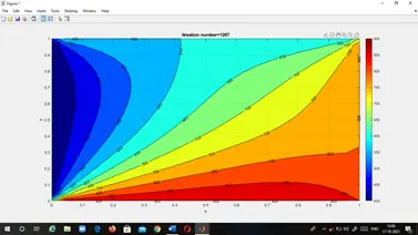
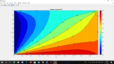
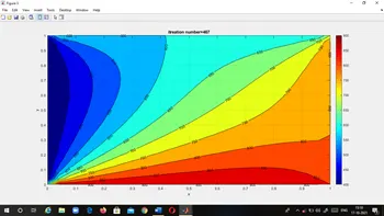
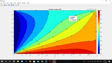
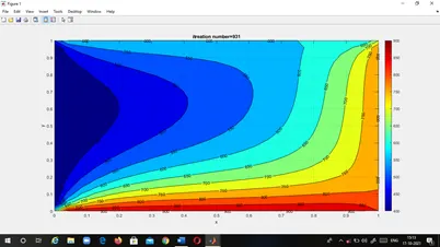
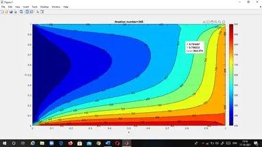
Output graphs-
1.steady state
I)Jacobian iteration
II)Gauss seidel iteration
III)Successive over relaxation iteration
2)Unsteady state-
Explicit
Implicit
I)Jacobian iteration
II)Gauss seidel iteration
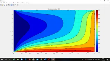
III)Successive over relaxation iteration
Results and conclusion
1.Results
|
Iterative solver |
Steady state |
Unsteady State |
|||
|
Explicit |
Implicit |
||||
|
Iteration number |
Simulation time |
In Explicit we don’t used iterative solver Iteration number=1001 Simulation time=0.0479 |
Iteration number |
Simulation time |
|
|
Jacobian |
1267 |
0.0545 |
931 |
0.0544 |
|
|
Gauss seidel |
677 |
0.0277 |
500 |
0.0326 |
|
|
Successive over relaxion |
467 |
0.0233 |
345 |
0.0266 |
|
2.Conclusion
From above chart and output graphs we conclude that successive over relaxation iteration method has faster convergence rate than remaining two method and we also say that Jacobian method has slowest among three method for converge the result of 2D heat conduction equation