Week 3.5 - Deriving 4th order approximation of a 2nd order derivative using Taylor Table method
Assignment Name-Deriving 4th order approximation of a 2nd order derivative using Taylor table method
Aim- Deriving 4th order approximation of a 2nd order derivative using Taylor table method
Objective-Deriving second order derivative by analytically and compare with three numerical approximation that you have derived
Given data-
f(x)=exp(x)*cos(x)
Number of nodes-
n=p+q (for one sided skewed scheme)
n=p+q-1 (for centre difference scheme)
Where,
n=number of nodes
p=order of derivative
q=order of approximation
Skewed System
Right side Skewed System
n=2+4
n=6
f''(x)=(af(x)+bf(x+dx) +cf(x+2dx)+df(x+3dx)+ef(x+4dx)+gf(x+5dx))/(dx^2)
left side skewed System
n=2+4
n=6
f''(x)=(af(x)+bf(x-dx) +cf(x-2dx)+df(x-3dx)+ef(x-4dx)+gf(x-5dx))/(dx^2)
centre Scheme
n=2+4-1
n=5
f''(x)=(af(x)+bf(x-dx) +cf(x-2dx)+df(x+dx)+ef(x+2dx))/(dx^2)
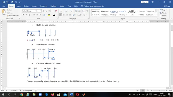
Analytical solution
f(x)=exp(x)cosx
=exp(x)cosx - exp(x)sinx
=exp(x)cosx - exp(x)sinx -exp(x)sinx - exp(x)cos(x)
= -2exp(x)sinx
Right skewed Scheme
Taylor table
|
f(i) |
Δxf’(i) |
Δx^2f’’(i) |
Δ^3f’’’(i) |
Δ^4f’’’’(i) |
|
|
f(i) |
a |
0 |
0 |
0 |
0 |
|
f(i+1) |
b |
b |
b/2 |
b/6 |
b/24 |
|
f(i+2) |
c |
2c |
2c |
8c/6 |
16c/24 |
|
f(i+3) |
d |
3d |
9d/2 |
27d/6 |
81d/24 |
|
f(i+4) |
e |
4e |
16e/2 |
64e/6 |
256e/24 |
|
f(i+5) |
g |
5g |
25g/2 |
125g/6 |
625g/24 |
|
sum |
0 |
0 |
1 |
0 |
0 |
Equations
a+b+c+d+e+g=0
b+2c+3d+4e+5g=0
b/2 +2c +9d/2 +16e/2 +25g/2=1
b/6+8c/6+27d/6+64e/6+125g/6=0
b/24+16c/24+81d/24+256e/24+625g/24=0
MATLAB code for solving matrix to find value of a, b, c, d, e, g
clear all
close all
clc
A=[1 1 1 1 1 1;0 1 2 3 4 5;0 1/2 2 9/2 16/2 25/2;0 1/6 8/6 27/6 64/6 125/6;0 1/24 16/24 81/24 256/24 625/24];
B=[0;0;1;0;0];
x=A\B;
Ans a= 1.9667 b= -3.9167 c=0 d=4.8333 e= -3.8333 g=0.9500
Left skewed scheme
Taylor table
|
f(i) |
Δxf’(i) |
Δx^2f’’(i) |
Δ^3f’’’(i) |
Δ^4f’’’’(i) |
|
|
f(i) |
a |
0 |
0 |
0 |
0 |
|
f(i+1) |
b |
-b |
b/2 |
-b/6 |
b/24 |
|
f(i+2) |
c |
-2c |
2c |
-8c/6 |
16c/24 |
|
f(i+3) |
d |
-3d |
9d/2 |
-27d/6 |
81d/24 |
|
f(i+4) |
e |
-4e |
16e/2 |
-64e/6 |
256e/24 |
|
f(i+5) |
g |
-5g |
25g/2 |
-125g/6 |
625g/24 |
|
sum |
0 |
0 |
1 |
0 |
0 |
Equation
a+b+c+d+e+g=0
-(b+2c+3d+4e+5g) =0
b/2 +2c +9d/2 +16e/2 +25g/2=1
-(b/6+8c/6+27d/6+64e/6+125g/6) =0
b/24+16c/24+81d/24+256e/24+625g/24=0
MATLAB code for solving matrix to find value of a, b, c, d, e, g
clear all
close all
clc
A=[1 1 1 1 1 1;0 -1 -2 -3 -4 -5;0 1/2 2 9/2 16/2 25/2;0 -1/6 -8/6 -27/6 -64/6 -125/6;0 1/24 16/24 81/24 256/24 625/24];
B=[0;0;1;0;0];
x=A\B;
Ans a= 1.9667 b= -3.9167 c=0 d=4.8333 e= -3.8333 g=0.9500
Centre Scheme
Taylor table
|
f(i) |
Δxf’(i) |
Δx^2f’’(i) |
Δ^3f’’’(i) |
Δ^4f’’’’(i) |
|
|
f(i-2) |
c |
-2c |
4c/2 |
-8c/6 |
16c/24 |
|
f(i-1) |
b |
-b |
b/2 |
-b/6 |
b/24 |
|
f(i) |
a |
0 |
0 |
0 |
0 |
|
f(i+1) |
d |
d |
d/2 |
d/6 |
d/24 |
|
f(i+2) |
e |
2e |
4e/2 |
8e/6 |
16e/24 |
|
sum |
0 |
0 |
1 |
0 |
0 |
equations
c+b+a+d+e=0
-2c-b+d+2e=0
4c/2+b/2+d/2+4e/2=1
-8c/6-b/6+d/6+8e/6=0
16c/24+b/24+d/24+16e/24=0
MATLAB code for solving matrix to find value of a,b,c,d,e
clear all
close all
clc
A=[1 1 1 1 1 ;-2 -1 0 1 2;4/2 1/2 0 1/2 4/2;-8/6 -1/6 0 1/6 8/6;16/24 1/24 0 1/24 16/24];
B=[0;0;1;0;0];
x=A\B;
Ans c=-0.0833 b=1.3333 a= -2.5000 d=1.3333 e =-0.0833
Function defining MATLAB code
Right Skewed Scheme
function error=right_skewed_scheme(x,dx);
%analytical function =exp(x)*cosx
%second derivative=-2*exp(x)*sinx
analytical_function= -2*exp(x)*sin(x);
%by using right skewed method
%f''(x)=(af(x)+bf(x+dx)+cf(x+2dx)+df(x+3dx)+ef(x+4dx)+gf(x+5dx))/dx^2
%consider
%t1=af(x),t2=bf(x+dx),t3=cf(x+2dx),t4=df(x+3dx),t5=ef(x+4dx),t6=gf(x+5dx)
t1=1.9667*exp(x)*cos(x);
t2=-3.9167*exp(x+dx)*cos(x+dx);
t3=0*exp(x+2*dx)*cos(x+2*dx);
t4=4.8333*exp(x+3*dx)*cos(x+3*dx);
t5=-3.8333*exp(x+4*dx)*cos(x+4*dx);
t6=0.9500*exp(x+5*dx)*cos(x+5*dx);
right_skewed_method=(t1+t2+t3+t4+t5+t6)/(dx^2);
%trunkage error
error=abs(right_skewed_method-analytical_function);
end
Left skewed scheme
function error=left_skewed_scheme(x,dx);
%analytical function =exp(x)*cosx
%second derivative=-2*exp(x)*sinx
analytical_function= -2*exp(x)*sin(x);
%by using left skewed method
%f''(x)=(af(x)+bf(x-dx)+cf(x-2dx)+df(x-3dx)+ef(x-4dx)+gf(x-5dx))/dx^2
%consider
%t1=af(x),t2=bf(x-dx),t3=cf(x-2dx),t4=df(x-3dx),t5=ef(x-4dx),t6=gf(x-5dx)
t1=1.9667*exp(x)*cos(x);
t2=-3.9167*exp(x-dx)*cos(x-dx);
t3=0*exp(x-2*dx)*cos(x-2*dx);
t4=4.8333*exp(x-3*dx)*cos(x-3*dx);
t5=-3.8333*exp(x-4*dx)*cos(x-4*dx);
t6=0.9500*exp(x-5*dx)*cos(x-5*dx);
left_skewed_method=(t1+t2+t3+t4+t5+t6)/(dx^2);
%trunkage error
error=abs(left_skewed_method-analytical_function);
end
centre Scheme
function error=centre_scheme(x,dx);
%analytical function =exp(x)*cosx
%second derivative=-2*exp(x)*sinx
analytical_function= -2*exp(x)*sin(x);
%by using centre method
%f''(x)=(af(x)+bf(x+dx)+cf(x+2dx)+df(x+3dx)+ef(x+4dx))/dx^2
%consider
%t1=af(x),t2=bf(x-dx),t3=cf(x-2dx),t4=df(x+dx),t5=ef(x+2dx)
t1=-2.5000*exp(x)*cos(x);
t2=1.3333*exp(x-dx)*cos(x-dx);
t3=-0.0833*exp(x-2*dx)*cos(x-2*dx);
t4=1.3333*exp(x+dx)*cos(x+dx);
t5=-0.0833*exp(x+2*dx)*cos(x+2*dx);
centre_method=(t1+t2+t3+t4+t5)/(dx^2);
%trunkage error
error=abs(centre_method-analytical_function);
end
Main MATLAB code for defining error
clear all
close all
clc
%input varibles
x=pi/3;
dx=linspace(pi/4,pi/4000,20);
%for loop
for i=(1:length(dx))
diff_right(i)=right_skewed_scheme(x,dx(i));
diff_left(i)=left_skewed_scheme(x,dx(i));
diff_centre(i)=centre_scheme(x,dx(i));
end
plot(dx,diff_right,'r')
hold on
plot(dx,diff_left,'b')
hold on
plot(dx,diff_centre,'g')
hold off
xlabel('grid size')
ylabel('error')
legend('right skewed scheme','left skeweds cheme','centre scheme')
Graphs
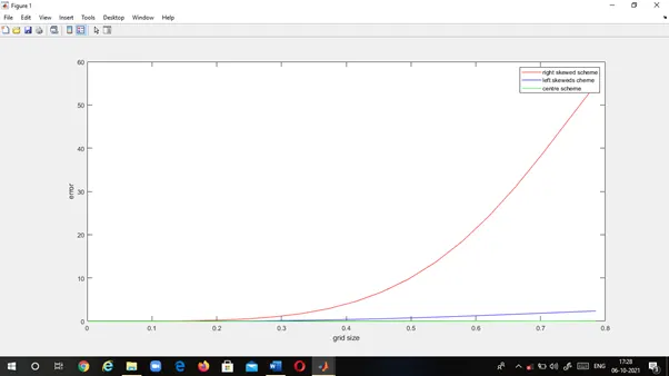
By using plot command
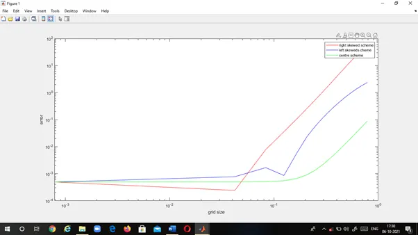
By using loglog command-
Only edit loglog instead of plot command in main MATLAB code for defining error
Before run the program be careful only change loglog
Conclusion-
We can see in both graph centre scheme has minimum error as compare to right and left skewed scheme. This obtain due to centre scheme collect the data from both side but CD scheme has some drawbacks are as follows
1.If any system does not have enough data or information from both side then we will used skewed scheme difference because of that Skewed scheme is useful
2.CD scheme cannot be employed at the boundary because unavailability of nodes at right and left side. In such situation CD scheme cannot do and skewed scheme do