Week 4 - CHT Analysis on Exhaust port

Aim:

To run simulation to anlyse Conjugate Heat transfer in Exhaust port.

Objective:

1.To understand why and where a CHT analysis is used.

2.Run the CHT simulation using different turbulence model and justify results.

Introduction:

Conjugate Heat Transfer (CHT):

The Conjugate Heat Transfer (CHT) analysis type allows for the simulation of heat transfer between solid and fluid domains by exchanging thermal energy at the interfaces between them.

where a CHT analysis is used

Internal Combustion Engines

The internal combustion engine industry is moving toward simulating the entire system rather than independent components. The accuracy of the predicted combustion in the cylinder is dependent on the temperature boundary conditions in the cylinder. By considering heat transfer in the metal components (e.g., the cylinder head, liner, piston, etc.), the cylinder wall no longer has a user-specified temperature, but instead has temperatures predicted as part of the complete-system simulation. This makes the overall simulation results more predictive by reducing the dependence on assumed boundary conditions.

Electromobility

Effective cooling strategies are critical for various components of emobility systems. Electric motors have high power densities and thus generate a significant amount of heat. If a motor is not properly cooled, high temperatures in the motor can cause the demagnetization of the permanent magnets and the breakdown of the winding insulation.

Aftertreatment

Predicting and mitigating urea deposit formation is a key challenge in Urea/SCR aftertreatment systems. When urea-water solution is sprayed into the engine exhaust system, it impinges on the wall as a liquid film. The decomposition of urea and the formation of undesirable deposits are highly dependent on wall temperature, and the heat transfer between the film and the wall is important to capture. Predicting the wall temperature helps you identify areas that are vulnerable to wall deposition.

Pumps and Compressors

Resolving the spatially varying surface temperature distributions in pumps and compressors improves the accuracy of the simulation and provides useful temperature data. For example, in a twin screw compressor, thermal expansion affects the clearance between the rotors. If that effect is not captured, the simulations will incorrectly predict leakage flows and lower the accuracy of your results.

Heat transfer coefficient (h):

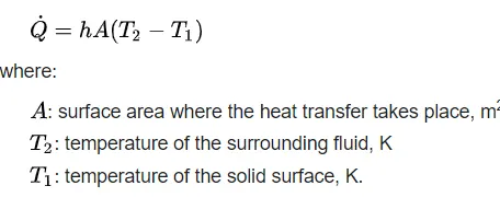
The heat transfer coefficient , in Thermodynamics is the proportionality constant between the heat flux and the thermodynamic driving force for the flow of heat

the heat transfer rate is:

Setup:

Geometry:

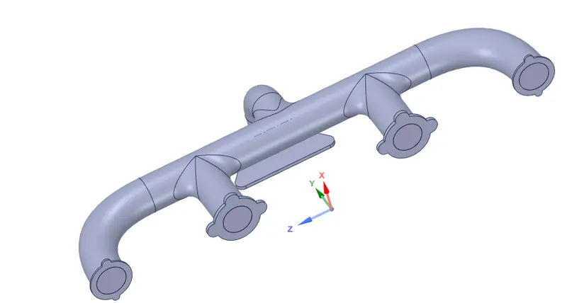
• Load the CAD model of Exhaust manifold in Spaceclaim and check for any extra edges, remove them if any.
• Go to Repair > Volume extract, and select the edges to separate inner and outer volume. Name the outer volume as Solid volume and inner ass Fluid volume and move bothe the volume to new component and delete empty components.
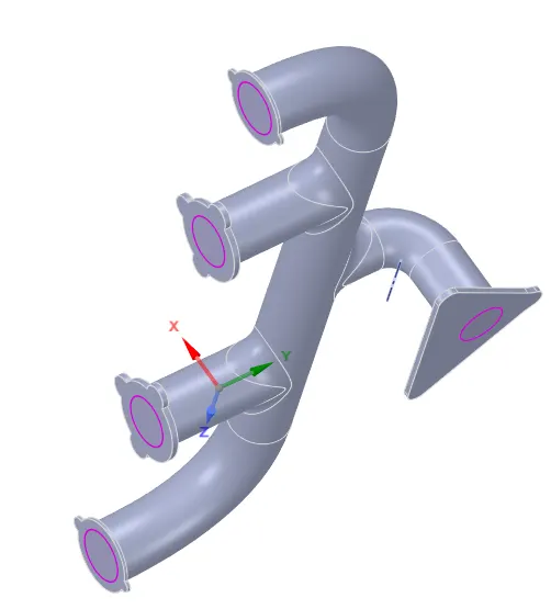
• Go to workbench > Shareprep, to share the physics between the fluid and solid volume and conformal mesh can be achieved.pink circle are seen after completing the procces.

Mesh:

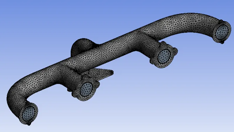
Open the mesh tab and select the geometry and named the parts.

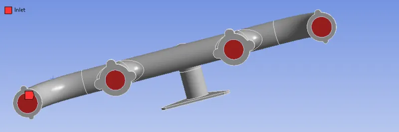
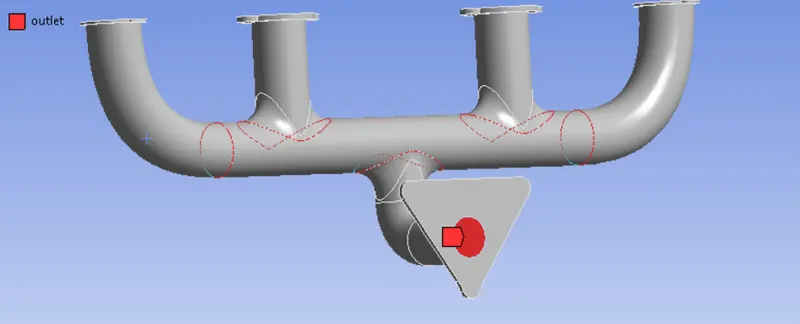
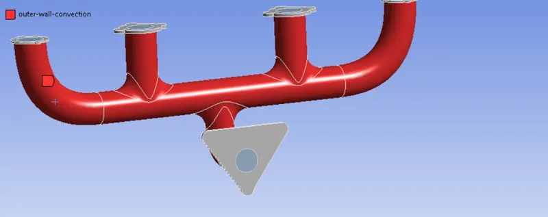
Ansys fluent automaticaly add unnamed part as wall and adiabatic boundary condition is applied.

Select the mesh and generate base mesh of default size as 150 mm.

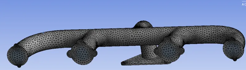
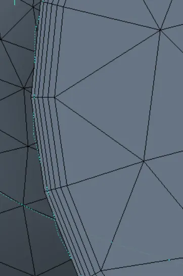
Now hide the outer body and select the inner face and named it as inflation layer.Go to inflation layer and select inflation layer and maximum thickness of 5 mm.

To refine the mesh size further, Go to mesh > sizing and add mesh size of 20 mm.

Solver:

Solver: Presure based steady state solver.

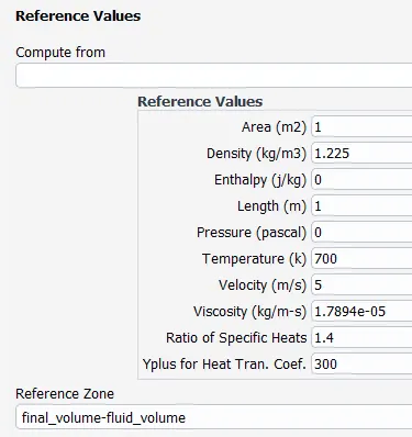
Refference Values:

Boundary Conditions:

Inlet:

Velocity = 5 m/s

Temperature = 700 K.

Outlet: Pressure = 0 Pa (Gauge pressure)

Outlet wall convection:

Thermal condition: Convection

Heat transfer coefficient = 20 W/m2K.

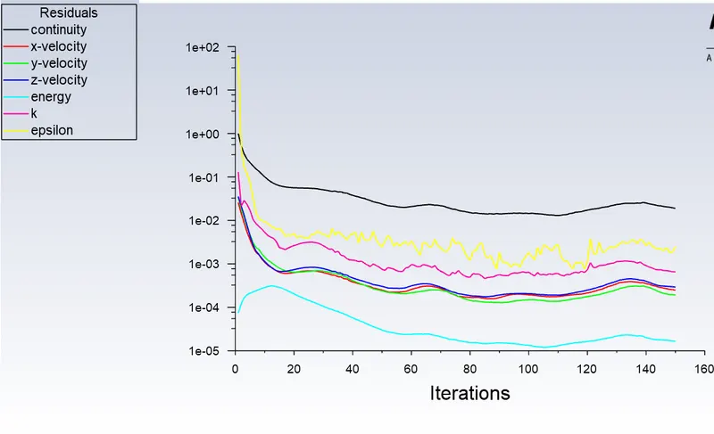
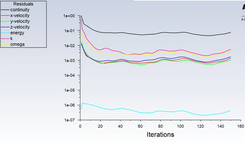
Simulation is ran for 150 iterations.

Results:

Case 1:

Mesh Size: 100 mm

Body sizing: 20 mm

Solver: K-epsilon standard

Mesh:

Residue Plot:

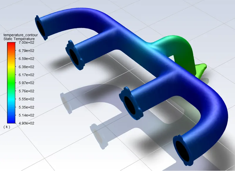
Temperature Contour:

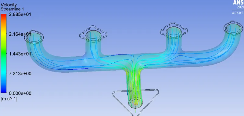
Velocity Steamlines:

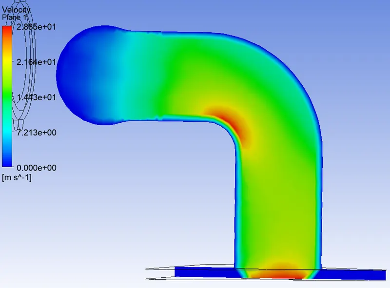
maximum velocity is 28.85 m/s and maximum velocity occured at outlet port.

Wall Heat transfer coefficient:

Case 2:

Mesh Size: 100 mm

Body sizing: 20 mm

Solver: K-epsilon Reliazable

Mesh:

Residue Plot:

Temperature Contour:

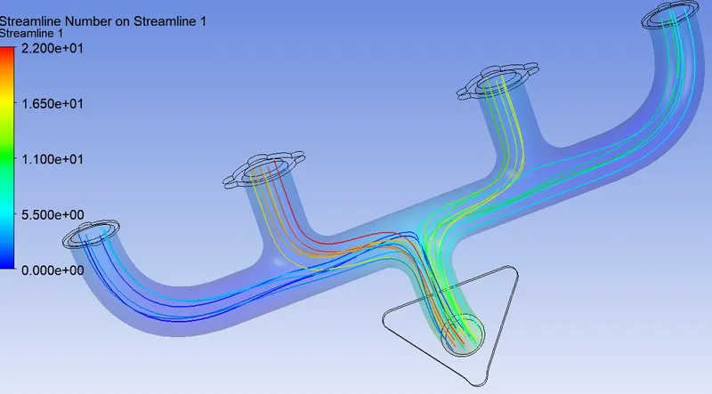
Velocity Steamlines:

maximum velocity is 22.00 m/s and maximum velocity occured at outlet port.

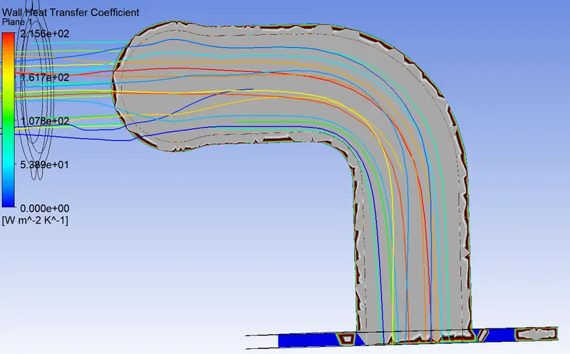
Wall Heat transfer coefficient:

Case 3:

Mesh Size: 100 mm

Body sizing: 20 mm

Solver: K-Omega

Mesh:

Residue Plot:

Temperature Contour:

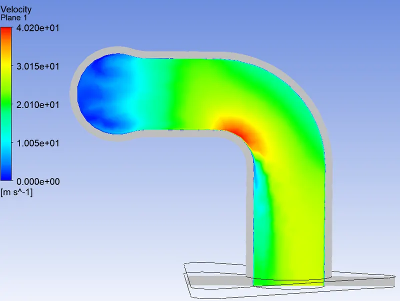
Velocity Steamlines:

maximum velocity is 40.20 m/s and maximum velocity occured at outlet port.

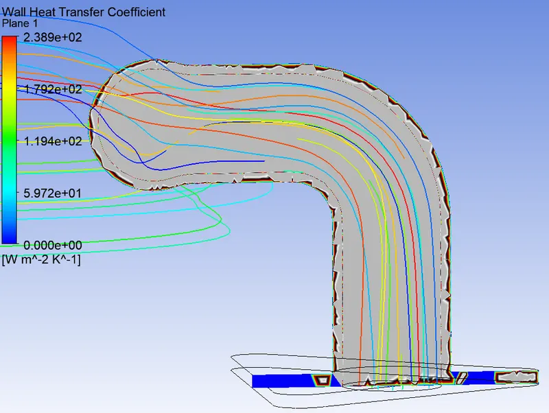
Wall Heat transfer coefficient:

Result Discussion:

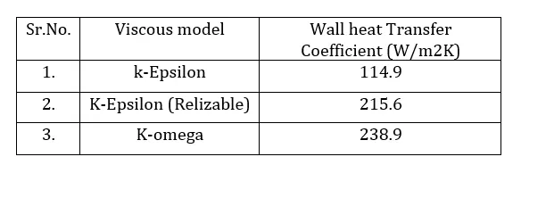
Wall heat transfer coefficient fro different viscous model is tabulated as follow:

• No difference in Temperature contours for all three viscous model is observed.
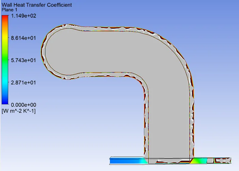
• Maximum heat transfer coefficient is found at layer adjacent to where maximum velocity is found.
• Maximum wall heat transfer is found using k-omega viscous model.

How would you verify if the HTC predictions from the simulations are right? On what factors does the accuracy of the prediction depend on?

The typical flow conditions in automotive exhaust systems produce Re numbers in the range of 10^3 to 5*10^4 . The exhaust flow often enters the region Re< 2300, especially in the exhaust manifold runners. In spite of that, the flow remains actually turbulent, since it has flowed through a substantial restriction. The exhaust valves and the persisting, unsteady, flow pulsation effects do not favour the transition to the laminar region

According to the Sieder Tate relation which correlates the Nu number with Re and Pr

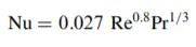
It means Nusselt no. is the function of Reynolds no. and Prandtl no.

As the turbulent boundary layer in the vicinity of bend at outlet port is thin maximum velocity of flow is observed at bend and hence higher Reynold no.

Now, Nu = h*L/K

As Length of pipe and thermal conductivity are constant, value of h will increases as Nu increases and Nu increases as Re increases.

As per our results, heat transfer coefficient is high for higher value of velocity and hence from above discussion we think that our results are correct.

Factors affects the quality of prediction:

• More refined mesh leads to the better results.
• Use inflation layers and apply proper Boundary condition.
• Proper selection of turbulence model according to y+ values.