Curve fitting using MATLAB

AIM:

To write a Profgrame using MATLAB to fit a linear and cubic polynomial for the given data

OBJECTIVE:

• write a code to fit a linear and cubic polynomial for the given data.
• plot the linear and cubic fit curves along with the raw data points.
• write a code to show the split wise parameters.
• Explain the parameters used to meausre the fitness charectrestics for bothe curves.

THEORY:

CURVE FITTING:

• Curve fitting is the process of constructing a curve or mathematical function,that has the best fit to a series of data points
• By curve fitting we can mathematically construct the functional relationship between the observed data and parameter values etc.
• It is also useful for the future predictions of the value which will be the one in future.
• Fitted curves can be used as an aid for data visualizations.

FITTING LINES AND POLYNOMIAL FUNCTIONS TO DATA POINTS:

• The first degree Polynomial equation

is a line with slope 'a'. A line will connect any two points, so a first degree polynomial equation is an exact fit through any two points with distinct x coordinates.

• If the order of the equation is increased to a second degree polynomial, the following results:

This will exactly fit a simple curve to three points.

• If the order of the equation is increased to a third degree polynomial, the following is obtained:

This will exactly fit four points.

PARAMETERS USED TO MEASURE THE FITNESS OF THE CURVE:

The parameters used to measure the fitness of the curve are

1. The sum of squares due to error(SSE).
2. R-square.
3. Adjusted R-square.
4. Root mean squared error(RMSE).

The sum of squares due to error(SSE): This static meausres the total deviation of the response values.It is also called the summed square of residuals and is usually labelled as SSE.

R-square: The quantity that measures how succesful the fit is in explaining the variation of the data.Put another way R-square is the square of the corrolation between the response values and predicted response values.It is also called as the square of the multiple correlation coefficient and the coefficient of multiple determination.

R-sqaure is defined as the ratio of sum of the regression to the total sum of squares

R-square ranges from any value between 0-1

• 0 for the worst possible fit
• 1 for the best possible fit

Adjusted R-square: Adjusted R-square: Adjusted r-square is a normalizing variation due to insignificant indipendent variable in R-square

Where,

n = number of data points

k = number of independent variables

Root mean squared error(RMSE): This static is also known as the fit standard error and the standard error of the regression.It is an estimate of the standard deviation of the random component in the data and is defined as,

Here, n = total number of data points

"Using these four quantities MATLAB effectively deduces the goodness of fit, typically is R-square is greater than 0.95 the fit is assumed to be good"

PROGRAMME:

LINEAR FIT:

STEP WISE EXPLANATION:

• The data of specific heat and temperature is loaded with the command "load" which is defined as "Cp_data".
• The Temperature and specific heat data are taken from the Cp_data.

cp_data = load('data');
temperature = cp_data(:,1);
cp = cp_data(:,2);

• To perform the curvefit there are two functions which is to be used i.e "polyfit" anad "polyval"
• "polyfit" is a matlab function used to compute the least square polynomial for a given set of data.polyfit genrates the coefficients which can be used for genrating the curve.
• "polyval" is used to evaluate the polynomial for given set of x values,so polyval genrate a curve fit the data based on the coefficients found using polyfit.
• using the polyval command the predicted_cp is obtained from the coefficients.

co_effs = polyfit(temperature,cp,2)
predicted_cp = polyval(co_effs,temperature)

• To plot the curve for original observed data for linear fit is

plot(temperature,cp,'linewidth',3)

• Now,to plot the curve fit the predicted cp and the temperature are used here
• The x and y labels are given with the specific heat and original data

plot(temperature,predicted_cp,'linewidth',3,'color','r')
xlabel('Temperature [k]')
ylabel('Specific heat [KJ/Kmol-k]')
legend('original data','curve fit')
title('linearfit')

OUTPUT:

LINEAR FIT:

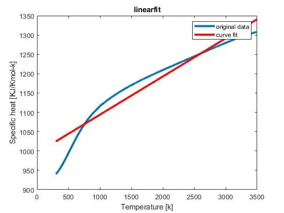
Here there are large variations between the two curves,Therefore they dont fit perfectly.

FOR CUBIC FIT:

• The code follows the same procedure until the coefiicients of the given parameters which is changed from one degree polynomial to three degree polynomial while cjanging the number in co_effs from 1 to 3
• The code the follows the same again as the linear one after the above steps

co_effs = polyfit(temperature,cp,3)
predicted_cp = polyval(co_effs,temperature)
plot(temperature,cp,'linewidth',3)
hold on
plot(temperature,predicted_cp,'linewidth',3,'color','r')
xlabel('Temperature [k]')
ylabel('Specific heat [KJ/Kmol-k]')
legend('original data','curve fit')
title('Cubicfit')

OUTPUT:

CUBIC FIT:

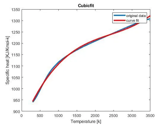
The is a very less difference between the curves and Therfore the curves are perfectly fit.

In Both the plots the curve fit is compared to the original data by plotting the linear and cubic fit.

FINAL FULL CODE:

FOR LINEAR FIT:

clear all
close all
clc
cp_data = load('data');
temperature = cp_data(:,1);
cp = cp_data(:,2);
%curve fit
% cp = a*T^2+b*T+c
co_effs = polyfit(temperature,cp,1)
predicted_cp = polyval(co_effs,temperature)
plot(temperature,cp,'linewidth',3)
hold on
plot(temperature,predicted_cp,'linewidth',3,'color','r')
xlabel('Temperature [k]')
ylabel('Specific heat [KJ/Kmol-k]')
legend('original data','curve fit')
title('Linear fit')

FINAL FULL CODE:

FOR CUBIC FIT:

clear all
close all
clc
cp_data = load('data');
temperature = cp_data(:,1);
cp = cp_data(:,2);
%curve fit
% cp = a*T^2+b*T+c
co_effs = polyfit(temperature,cp,3)
predicted_cp = polyval(co_effs,temperature)
plot(temperature,cp,'linewidth',3)
hold on
plot(temperature,predicted_cp,'linewidth',3,'color','r')
xlabel('Temperature [k]')
ylabel('Specific heat [KJ/Kmol-k]')
legend('original data','curve fit')
title('Cubicfit')

TO check or Validate the fitness charactrestics:

NOTE: Curve fitting Toolbox in MATLAB is used to validate the fitness charactrestics.

CURVE FITTING TOOL BOX:

• Curve fitting tool box is another alternative way to validate the fitness charactrestics of the curve.We just have prepared the data first and then open the "Curve fitting tool box" in matlab and then select the X and Y values.
• The tool Box will automatically creates a curve,after that the degree of polynomial has to be selected to fit the original curve.This will plot a new curve according to the degree of polynomial as well as it will display Goodness of the fit in the left side of the box.

LINEAR FIT:

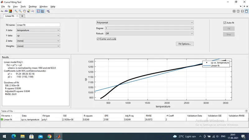
• Here in the above image in the left side corner there are the resukts shown below that the Goodness of fit is given in which the four Parameters are given
• And we can consider one of the parameter which could be the adjusted R-square
• Here we can see the Value of the Adjusted R-square is given as 0.9249 which can be 92.49%.
• The Linear Regression for Adjusted R-square is 92.49% which is not a good fit.

CUBIC FIT:

• Here we can see the Value of the Adjusted R-square is given as 0.9967 which can be 99.67%.
• The Linear Regression for Adjusted R-square is 99.67% which is a better fit.

After the research done using these methods and changing the parameters.

HOW TO MAKE CURVE FIT PERFECTLY:

• To get the perfect fit the R-square value should be exactly 1.This value is obtained only when both curves meet together perfectly.
• By increasing the order of polynomial in the curve fit tool box we can get to see the value of R-sqaure changes at a particular degree.
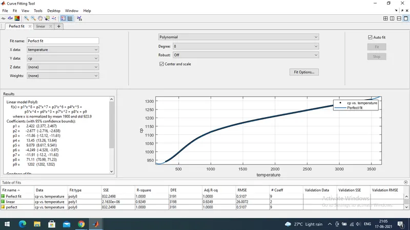
• For me i have been interpolating the datasets,by interpolating the errors are reduced here i have increased the polynomial degree until 8 where i have obtained the value of R-square as 1 exactly which is a perfect fit.

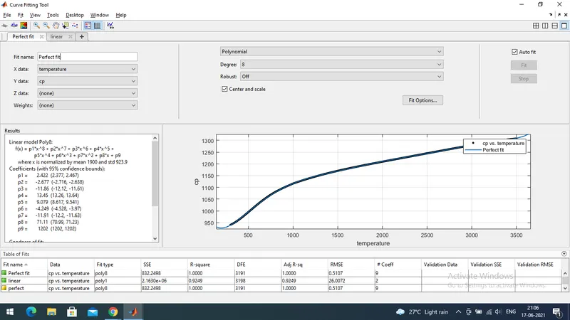
Here we can see the value of R-square is exactly equal to 1,where the degree of polynomial is 8.

HOW TO GET THE BEST FIT:

• The degree of polynomial effects the detail to which it approximates the data.
• A first degree polynomial is a simpler linear fit,The degree being less than the number of parameters the polynomial estimates.
• The higher the polynomial degree the closer the curve gests fit,lower degree has the effect pf the smoothing the fit,acting as a sort of low pass filter
• Altough the polynomial degree higher than 7 doesnt add any significant information.choosing the polynomial degree is the factor of experimenting the to determine what works the best.
• To see the effect of the polynomial degree, the easiest way is to experiment using polyval and polyfit with random data
• if we can observe one thing the third degree polynomial axproximates the sine curve,where the 9th degree polynomial fits the data more closely but does not at all approximates the sine curve.

WHAT COULD BE DONE TO IMOROVE THE CUBIC FIT:

• The cubic fit can be improved by splitting the curve fits into multiple number of polynomials for different set of temperature and the specififc heat.
• It can also be improved by reducing the erro between the original data case and curve fit value
• To improve the cubic fit data we can also split the data into many small data,Here i have used this method by taking four different subparts are as follows.

CODE WITH SPLITTING THE DATA TO IMPROVE THE CUBIC FIT:

STEP WISE EXPLANATION:

• The data is loaded and defined it as cp_data.
• The same procedure which is used for linear fit is followed here for the initial steps.

cp_data = load('data')
temperature = cp_data(:,1);
cp = cp_data(:,2);

• The data is splitted into 4 smaller data for both temperature and the Cp

%Splitting
temperature1 = cp_data(1:800,1)
cp1 = cp_data(1:800,2)
temperature2 = cp_data(801:1600,1)
cp2 = cp_data(801:1600,2)
temperature3 = cp_data(1601:2400,1)
cp3 = cp_data(1601:2400,2)
temperature4 = cp_data(2401:3200,1)
cp4 = cp_data(2401:3200,2)

• Coefficeint of the 4 parameters are obtained by the polyfit and polyval commands,with cubic polynomial into consideration.
• using ployfit and polyval both the coefficients and predicted cp are obtained.

co_effs1 = polyfit(temperature1,cp1,3)
co_effs2 = polyfit(temperature2,cp2,3)
co_effs3 = polyfit(temperature3,cp3,3)
co_effs4 = polyfit(temperature4,cp4,3)
predicted_cp1 = polyval(co_effs1,temperature1)
predicted_cp2 = polyval(co_effs2,temperature2)
predicted_cp3 = polyval(co_effs3,temperature3)
predicted_cp4 = polyval(co_effs4,temperature4)

• The curve fit for each individual and the curve for the original data is plotted

%plotting
%original data
plot(temperature,cp,'linewidth',3,'color','b')
hold on
%curve fit
plot(temperature1,predicted_cp1,'linewidth',3,'color','r')
hold on
plot(temperature2,predicted_cp2,'linewidth',3,'color','r')
hold on
plot(temperature3,predicted_cp3,'linewidth',3,'color','r')
hold on
plot(temperature4,predicted_cp4,'linewidth',3,'color','r')
xlabel('Temperature [k]')
ylabel('Specific heat [KJ/Kmol-k]')
legend('original data','curve fit')

OUTPUT:

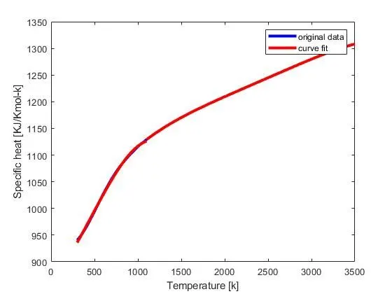
Here,By splitting the data we can see the difference between the curve is minimised where we get a better fit than the earlier cubic fit.

FINAL FULL CODE:

SPLITTING THE DATA FOR CUBIC FIT:

clear all
close all
clc
cp_data = load('data')
temperature = cp_data(:,1);
cp = cp_data(:,2);
%Splitting
temperature1 = cp_data(1:800,1)
cp1 = cp_data(1:800,2)
temperature2 = cp_data(801:1600,1)
cp2 = cp_data(801:1600,2)
temperature3 = cp_data(1601:2400,1)
cp3 = cp_data(1601:2400,2)
temperature4 = cp_data(2401:3200,1)
cp4 = cp_data(2401:3200,2)
%coefficient for the 4 different parameters
%cubic polynomial
% cp = a*T^3+b*T^2+c*T+d
co_effs1 = polyfit(temperature1,cp1,3)
co_effs2 = polyfit(temperature2,cp2,3)
co_effs3 = polyfit(temperature3,cp3,3)
co_effs4 = polyfit(temperature4,cp4,3)

predicted_cp1 = polyval(co_effs1,temperature1)
predicted_cp2 = polyval(co_effs2,temperature2)
predicted_cp3 = polyval(co_effs3,temperature3)
predicted_cp4 = polyval(co_effs4,temperature4)
%plotting
%original data
plot(temperature,cp,'linewidth',3,'color','b')
hold on
%curve fit
plot(temperature1,predicted_cp1,'linewidth',3,'color','r')
hold on
plot(temperature2,predicted_cp2,'linewidth',3,'color','r')
hold on
plot(temperature3,predicted_cp3,'linewidth',3,'color','r')
hold on
plot(temperature4,predicted_cp4,'linewidth',3,'color','r')
xlabel('Temperature [k]')
ylabel('Specific heat [KJ/Kmol-k]')
legend('original data','curve fit')

ERRORS:

There are no Complicated or matheatical errors faced or found while executing all the programes used.

RESULTS AND CONCLUSION:

The MATLAB programme is written to fit the linear and cubic polynomials using the Cp data.

After performing i have obsserved there are many different ways used to get the curve fit perfect by considering the four parameters.

After splitting the Data i have found the if we can split the data into more number of smaller data we can get the better fit and better results.

Other than single degree or lower degree polynomial i guess and i found having the higher degree polynomials obtain the better output results.

REFERENCES:

• https://skill-lync.com/projects/Curve-Fitting-and-criterion-to-choose-best-fit-41860
• https://en.wikipedia.org/wiki/Curve_fitting
• https://in.mathworks.com/help/curvefit/curve-fitting.html