Air Standard Cycle using MATLAB
AIM:
TO write a code in MATLAB to solve the Otto cycle and Plot the PV-diagram.
OBJECTIVE:
- To write a code to solve the otto cycle.
- To understand the otto cycle analysis through MATLAB.
- To plot PV-diagram using this code.
- To find the thermal efficiency of the engine
THEORY:
An Otto cycle is an idealzed thermodynamic cycle that describes the functioning of a typical spark ignition piston engine.It is the thermodynamic cycle most commonly used in automobile engines.
1.This was first invented even before the diesel cycle.
2.This is an Air standard cycle (Working substance is air which behaves as ideal gas).
3.Substance is of mixed mass.Closed system analysis is done.
4.Gasoline is used as fuel.where the intake is the mixture of fuel and air.
5.Cp and Cv are constant all process are reversible.
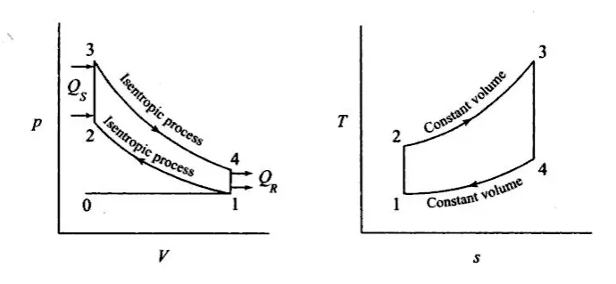
The otto cycle has all reversible processes
- process 1-2 = Adiabatic compression as the piston moves from bottom dead center(BDC) to top dead center(TDC).
- process 2-3 = constant volume heat addition to the source while the piston is on the top dead center(TDC).The ignition is initiated
- process 3-4 = Adiabatic Expansion which is power stroke
- process 4-1 = constant volume heat rejection where the air is rejected to the air when the piston is in bottom dead center(BDC).
Governing Equations:
Compression ratio(Cr) = 1+(Vs/Vc)
The optimum compression ratio is preferred
Change of volume inside the combustion chamber V = 1/2*(rc-1)*(R+1-cos(θ)-(R^2-sin(θ)^2)^1/2
Swept volume Vs = π/4*D^2*L
(where D = Bore,L= stroke)
Clearance volume Vc = swept volume/(Cr-1)
Ideal gas equation = PV/T = constant.
For isentropic Compression and Exoansion process => PV^gamma = T
Thermal efficiency:
where T is temperature in kelvin
P is pressure in pa, V is volume and gamma is specific heat ratio
R is Ratio of length of connecting rod to the crank pin radius
Crank pin radius is (a).
CODE:
EXPLANATION:
- First the inputs are given starting with engine parameters.
%geometric parameters of the engine
%stroke lenghth(m)
stroke = 0.1;
%bore diameter(m)
bore = 0.1;
%length of connecting rod(m)
c_rod = 0.15
%compression ratio
c_r = 12;
%specific heat ratio
gamma = 1.4;
- Compression ratio is given so the swept volume and clearance volume is found with which V1 and V2 is found through that.
%caluculating the swept volume
v_swept = (pi/4)*bore^2*stroke;
v_clearance = v_swept/(c_r-1);
v1 = v_swept+v_clearance;
v2 = v_clearance- The state variables at state point 1 is given.
%state variables at state point 1
p1 = 101325;
t1 = 500;- The state variables at state point 2 is the entered which is at the start of the combustion.
%state variables at state point 2
%p1v1^gamma = p2v2^gamma | p2 = p1*(v1/v2)^gamma
p2 = p1*(v1/v2)^gamma
%from ideal gas equation
%p1v1/t1 = p2v2/t2 | t2 = p2*v2*t1/p1*v1
t2 = (p2*v2*t1)/(p1*v1)
- The state variables at the state ponit 3 which is at the end of the combustion.
%sate variables at state point 3
v3 = v2
%from ideal gas equation
%p2v2/t2 = p3v3/t3 | p3 = p2*v2*t3/v3*t2
p3 = (p2*t3)/t2;
- The state variables at the state point 4 which is at the end of the power stroke.
%satet variables at state point 4
v4 = v1
%p4v4^gamma = p3v3^gamma | p4 = p3*(v3/v4)^gamma
p4 = p3*(v3/v4)^gamma
%p4v4/t4 = p1v1/t1 | t4 = p4*v4*t1/p1*v1
t4 = p4*v4*t1/p1*v1- Plotting the graphs using the above parameters.
%plotting PV
figure(1)
hold on
plot(v1,p1,'*','color','r')
plot(v2,p2,'*','color','b')
plot(v3,p3,'*','color','y')
plot(v4,p4,'*','color','g')
OUTPUT:
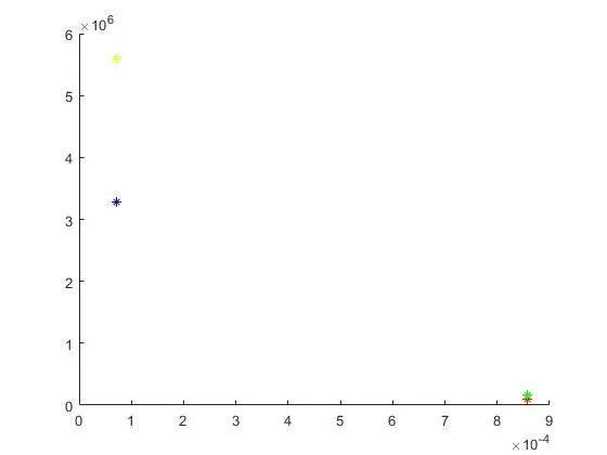
- In order to plot the paths we need to solve the piston kinematics,It actually tells us how the piston moves form BDC to TDC and also how the combustion volume changes.
- To determine the change of the volume inside the combustion chamber.
- Change of volume inside the combustion chamber
V = 1/2*(rc-1)*(R+1-cos(θ)-(R^2-sin(θ)^2)^1/2 ---- (1)
- For that function is used which intakes certain inputs to caluclate the volume of compression and expansion with the help of the equation (1).
function [V] = engine_kinematics(bore,stroke,c_rod,c_r,start_crank,end_crank)

a = stroke/2;
R = c_rod/a;
v_swept = (pi/4)*bore^2*stroke;
v_clearance = v_swept/(c_r-1);
theta = linspace(start_crank,end_crank,100);

term1 = 0.5*(c_r-1);
term2 = R+1-cosd(theta);
term3 = (R^2-sind(theta).^2).^0.5;

V = (1+term1*(term2-term3))*v_clearance
end
The volume inside the engine is going to vary.
To plot the paths for the isentropic compression and isentropic expansion from the above step a code has been written.
- For isentropic compression the code is.
c_constant = p1*v1^gamma
V_compression = engine_kinematics(bore,stroke,c_rod,c_r,180,0)
p_compression = c_constant./V_compression.^gamma
- For isentropic Expansion the code is.
c_constant = p3*v3^gamma
V_expansion = engine_kinematics(bore,stroke,c_rod,c_r,0,180)
p_expansion = c_constant./V_expansion.^gamma
- Now to plot those curve or path for the isentropic compression the code is given as
plot(V_compression,p_compression,'color','g','linewidth',3)- Now to plot the curve for the isentropic Expansion the code is given as
plot(V_expansion,p_expansion,'color','b','linewidth',3)
- To plot the remaining paths i.e, for constant volume heat addition and constant volume heat rejection
plot([v2 v3],[p2 p3],'color','r','linewidth',2)
plot([v4 v1],[p4 p1],'color','c','linewidth',2)
Therefore all the paths are formed through the above codes
Now to find the thermal efficiency of engine the following equation is used
ERRORS FACED:
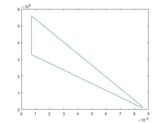
while trying to plot the phase for the isentropic compression and isentropic expansion without using a funiction an error has occured using this code
Plotting them gets a straight line which is wrong which is representing the wrong path.
figure(2)
plot([v1 v2 v3 v4 v1],[p1 p2 p3 p4 p1])
ERROR OCCURED WHILE PLOTTING THE PATHS:
FINAL CODE:
function [V] = engine_kinematics(bore,stroke,c_rod,c_r,start_crank,end_crank)

a = stroke/2;
R = c_rod/a;
v_swept = (pi/4)*bore^2*stroke;
v_clearance = v_swept/(c_r-1);
theta = linspace(start_crank,end_crank,100);

term1 = 0.5*(c_r-1);
term2 = R+1-cosd(theta);
term3 = (R^2-sind(theta).^2).^0.5;

V = (1+term1*(term2-term3))*v_clearance
end
MAIN CODE:
clear all
close all
clc

%inputs
t3 = 2300;
%state variables at state point 1
t1 = 500;
p1 = 101325;
%geometric parameteres of the engine
%bore diameter
bore = 0.1;
%stroke length
stroke = 0.1;
%length of connecting rod
c_rod = 0.15;
%compression ratio
c_r = 12;
%specific heat ratio
gamma = 1.4;

%caluculating the swept volume and clearance volume
v_swept = (pi/4)*bore^2*stroke;
v_clearance = v_swept/(c_r-1);
v1 = v_swept+v_clearance
v2 = v_clearance

%state variables at state point2
%p2v2^gamma = p1v1^gamma | p2 = p1*(v1/v2)^gamma
p2 = p1*(v1/v2)^gamma;
%from ideal gas equation p1v1/t1 = p2v2/t2
t2 = (p2*v2*t1)/(p1*v1);
c_constant = p1*v1^gamma
V_compression = engine_kinematics(bore,stroke,c_rod,c_r,180,0)
p_compression = c_constant./V_compression.^gamma


%state variables at state point 3
%due to constant volume
v3 = v2;
%p2v2/t2 = p3v3/t3 | p3 = p2*v2*t3/v3*t2
p3 = (p2*t3)/t2;
c_constant = p3*v3^gamma
V_expansion = engine_kinematics(bore,stroke,c_rod,c_r,0,180)
p_expansion = c_constant./V_expansion.^gamma


%state variables at state point 4
v4 = v1;
%p4v4^gamma = p3v3^gamma | p4 = p3*(v3/v4)^gamma
p4 = p3*(v3/v4)^gamma;
%p4v4/t4 = p1v1/t1 | t4 = p4*v4*t1/p1*v1
t4 = p4*v4*t1/p1*v1

%thermal efficiency
eff = (1-1/c_r^(gamma-1))*100


%plotting PV
figure(1)
hold on
plot(v1,p1,'*','color','r')
plot(V_compression,p_compression,'color','g','linewidth',2)
plot(v2,p2,'*','color','b')
plot([v2 v3],[p2 p3],'color','r','linewidth',2)
plot(v3,p3,'*','color','y')
plot(V_expansion,p_expansion,'color','b','linewidth',2)
plot(v4,p4,'*','color','g')
plot([v4 v1],[p4 p1],'color','c','linewidth',2)
title('otto cycle')
legend("initial state","isentropic compression","before heat addition","isochoric heat addition","before expansion","isentropic expansion","before exhaust","isochoric heat rejection")
xlabel('volume')
ylabel('pressure')
grid on
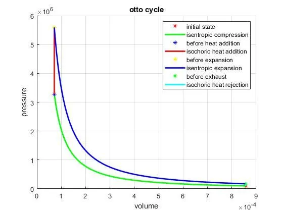
OUTPUT:
P-V daigram
THERMAL EFFICIENCY:
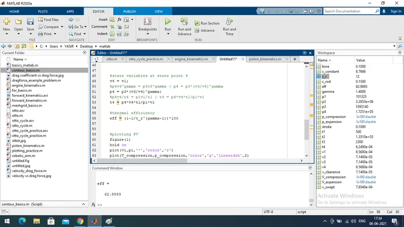
eff =62.9893
RESULT AND CONCLUSION:
- Hence,The code is compiled succesfully using MATLAB.
- The code has created the PV diagram succesfully considering the errors too
- The output for the thermal efficiency of the egine is 62.9893.
- The erros are also uploaded
- The final output for PV diagram and the efficiency is also uploaded