Solving second order ODEs using MATLAB

The simple pendulum is a mechanical system that moves in an oscillatory motion. It consists of a point mass 'm' suspended by means of light inextensible string of length L from a fixed support.The motion occurs in a vertical plane and is driven by a gravitational force 'g'.

The period of swing of a simple pendulum depends on its length, the gravity and to a small extent on the maximum angle that the pendulum swings away from vertical, θ₀, called the amplitude It is independent of the Mass of the bob.

When the Bob is in equilibrium it is subjected to an external force which displaces from its intial position and oscillates in a circualr arc in the same vertical plane.

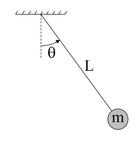
In Engineering, ODE is used to describe the transient behavior of a system.

The way the pendulum moves depends on the Newtons second law. When this law is written down, we get a second order Ordinary Differential Equation that describes the position of the bob w.r.t time.

The motion can be shown through this coding form using the MATLAB.

EQUATION:

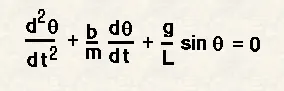
In the above equation,

g = gravity in m/s2, = 9.81 m/s^2

L = length of the pendulum in m, = 1m

m = mass of the ball in kg, = 1kg

b = damping coefficient. = 0.05

Angular displacement = 0

Angular velocity = 3rad/sec

DETAILED EXPLANATION OF CODE:

CODE:

• First the inputs are given.

%inputs
%damping coefficient
b = 0.05;
%gravity m/s^2
g = 9.81;
%length of the pendulum string;Metre
l = 1;
%mass kg
m = 1;

• for solving first ODE it is required to provide the value for dispalcement and velocity.
• Initial displacement is 0.
• initial velocity is 3.
• Time intervals are also provided.
• Therefore the initial conditions are given as.

%initial condition
theta_0 = [0 3]; %initial value for both velocity and displacement
%time points
t_span = linspace(0,20,100);

• Calling the ODE function.
• The theta1 and theta2 values are provided inside the function parameter.
• dtheta1_dt and dtheta2_dt values are also given.
• The two values are labelled as single output which is dtheta_dt.

function [dtheta_dt] = ode_func(t,theta,b,g,l,m)

theta1 = theta(1)
theta2 = theta(2)
dtheta1_dt = theta2;
dtheta2_dt = -(b/m)*theta2-(g/l)*sin(theta1);
dtheta_dt = [dtheta1_dt;dtheta2_dt];
end

• Solving the ODE by calling the above function in it.
• Here t and theta are two anonymous values which is insertd inside the code using a variable '@'
• ode_func is called from the above function.
• Then the initial conditions are followed by them.

%solving ODE
[t,results] = ode45(@(t,theta)ode_func(t,theta,b,g,l,m),t_span,theta_0)

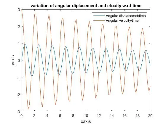
• Through the above parameters a graph is plotted to show the variation of displacement and velocity with respect to the time.

figure(1)
plot(t,results(:,1))
hold on
plot(t,results(:,2))
hold off
xlabel('xaxis')
ylabel('yaxis')
legend('Angular displacemet/time','Angular velocity/time')
title('variation of angular diplacement and elocity w.r.t time')

OUTPUT:

• Figure(1)

Commands for plotting the motion of a pendulum

• Contour command is used to change loop iteration after every motion.
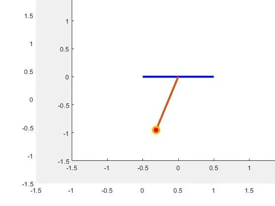
• X=0,y=0 depicts initial condition of pendulum bob.
• For loop is used to genrate the repeated conditions of the provided paremeters.
• Using the marker command we can attach the bob to the string.

ct = 1
for i = 1:length(theta2)
    THETA2 = theta2(i)
    x0 = 0;
    y0 = 0;
    x1 = l*sin(THETA2)
    y1 = -l*cos(THETA2)
    figure(2)
    plot([-0.5 0.5],[0 0],'color','b','linewidth',3)
    hold on
    plot([x0 x1],[y0 y1],x1,y1,'o','markers',10,'markerfacecolor','r','linewidth',3)
    axis([-1.5 1.5 -1.5 1.5])
    pause(0.002)
    hold off
    M(ct) = getframe(gcf)
    ct = ct+1
end

OUTPUT:

• FIGURE(2)

ANIMATION:

Commands for genrating animation

• In MATLAB when compared to OCTAVE it is very simple to create an animation by just using the VideoWriter command.
• The M is the movie and getframe is used to capture each and every frame in it.
• FInally all the frames are captured and executed using the videofile command in and uncompressed form
• Movie of M is saved and then animation is genrated through videofile using the videowriter command

movie(M)
videofile = VideoWriter('simple_pendulum.avi','uncompressed AVI')
open(videofile)
writeVideo(videofile,M)
close(videofile)

ERRORS:

While writing the function code i have used ; instead of , between dtheta1_dt and dtheta2_dt which where i faced a problem.

It should be a row and column vector but i have given , which makes it as a complete row vector only.

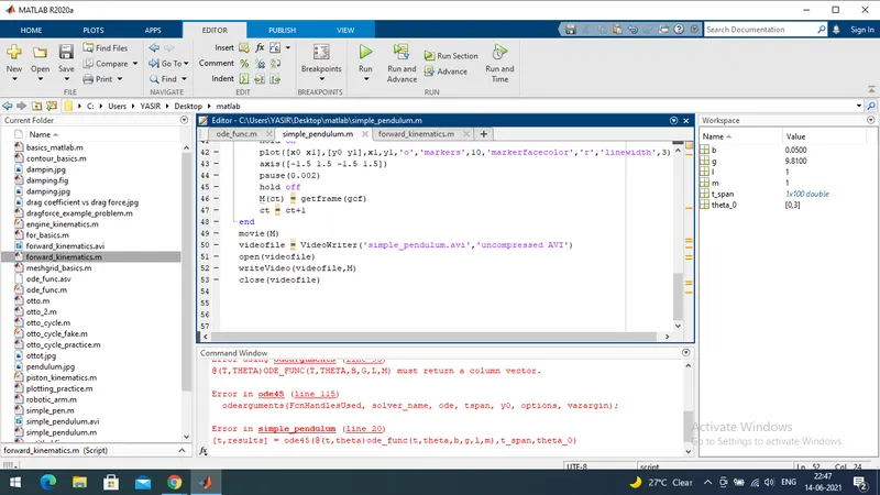
I have just changed the , with ; that's it everything got back to its way perfectly.

FINAL CODE:

CODE(1)

function [dtheta_dt] = ode_func(t,theta,b,g,l,m)

theta1 = theta(1)
theta2 = theta(2)
dtheta1_dt = theta2;
dtheta2_dt = -(b/m)*theta2-(g/l)*sin(theta1);
dtheta_dt = [dtheta1_dt;dtheta2_dt];
end

MAIN CODE:

clear all
close all
clc

%inputs
%damping coefficient
b = 0.05;
%gravity m/s^2
g = 9.81;
%length of the pendulum string;Metre
l = 1;
%mass kg
m = 1;

%initial condition
theta_0 = [0 3]; %initial value for both velocity and displacement
%time points
t_span = linspace(0,20,100);
%solving ODE
[t,results] = ode45(@(t,theta)ode_func(t,theta,b,g,l,m),t_span,theta_0)
%plotting damping graph
figure(1)
plot(t,results(:,1))
hold on
plot(t,results(:,2))
hold off
xlabel('xaxis')
ylabel('yaxis')
legend('Angular displacemet/time','Angular velocity/time')
title('variation of angular diplacement and elocity w.r.t time')
theta2 = results(:,1)
ct = 1
for i = 1:length(theta2)
    THETA2 = theta2(i)
    x0 = 0;
    y0 = 0;
    x1 = l*sin(THETA2)
    y1 = -l*cos(THETA2)
    figure(2)
    plot([-0.5 0.5],[0 0],'color','b','linewidth',3)
    hold on
    plot([x0 x1],[y0 y1],x1,y1,'o','markers',10,'markerfacecolor','r','linewidth',3)
    axis([-1.5 1.5 -1.5 1.5])
    pause(0.002)
    hold off
    M(ct) = getframe(gcf)
    ct = ct+1
end
movie(M)
videofile = VideoWriter('simple_pendulum.avi','uncompressed AVI')
open(videofile)
writeVideo(videofile,M)
close(videofile)

    

OUTPUT:

https://youtu.be/am4CHMF0SMg

RESULTS AND CONCLUSION:

• A MATLAB program is written that solves the ODE.
• A plot is made which shows the variation of displacement and velocity with respect to the time.
• The motion of the simple pendulum is shown using the MATLAB program.
• The errors are shown using the image.

THANK YOU