Genetic Algorithm to optimize the stalagmite Function
AIM:
To write a code using MATLAB to optimize the stalagmite function and find the global maxima of the function.
OBJECTIVE:
To write a code in MATLAB to optimize the stalagmite function.
Undersrand and Explain the concept of genetic algorithm in MATLAB.
Plot graphs for all three studies and for Fmaximum vs No of iterations.
THEORY:
Optimization:
- Optimization is used for mathematical programming such as MATLAB which is a process of selection of a best element with regard to some criteria.
- ]Optimization is done by systematically choosing input values from within an allowed set and computing the results of the function
Stalagmite Function:
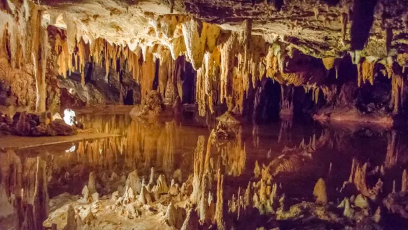
- A stalagmite is an upward growing mound of mineral deposits that have precipitated from water dripping on to the floor of a cave.Most stalagmites have rounded or flatted tips.
- A stalagmite function genrally refers to function with which we are genrating values over a stalagmite kind of surface for finding out the local and global maxima and minima of that particular given function.
- In MATLAB to perform optimization we use genetic algorithm method which is an inbuilt function to find the global maxima and minima of that given stalagmite function.
Genetic Algorithm:
- Genetic algorithm is an optimization technique use to solve Non-linear & Non-Differential optimization problems.This was came form using the revolutionary technique of Darwin Theory.
- The technique of the optimization is develope by john holland and his university student of Univerity of Michigan.
- This algorithm reflects the process of natural selection where the fittest individuals are served for reproduction in order to produce the offspring of next genration.
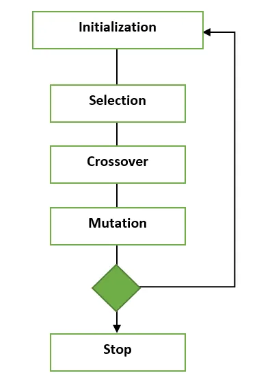
- Five phases are considered in genetic algorithm They are:
- Initial Population
- Fitness Function
- Slection
- Cross over
- Mutuation
*Initial Population:
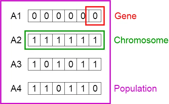
- The process begins with set of individuals which is called population.Each individual is a solution to the problem you want to solve.
- An individual is charactrized by set of parameters known as genes.They are joined into a string to form a chromosome.
*Caluculate Fitness:
- The fitness function determines how fit and individual is.It gives a fitness score to each individual.The probability that an individual will be selected for reproduction is based on its fitness score.
*Selection:
- The idea of selection phase is to select the first individuals and let them pass their genes to the next genration.
- Two pairs of individuals are selected based on their fitness scores.Individuals with high fitness score have more chance to be selected for reproduction.
*Crossover:
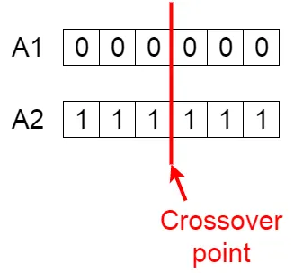
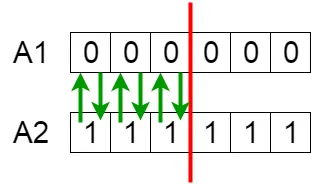
- Cross over is the most siginficant phase in genetic algorithm.For each pair of parents to be matted, a crossover point choosen at rand from within the genes.
*Mutuation:
- In certain new offspring is formed, some of their genes can be subjected to a mutuation with low random probability.This implies that some of the bits in the bit string can be flipped.
SYNTAX FOR GA:
x = ga(fun,nvars) finds a local unconstrained minimum, x, to the objective function, fun. nvars is the dimension (number of design variables) of fun.
x = ga(fun,nvars,A,b) finds a local minimum x to fun, subject to the linear inequalities A*x ≤ b. ga evaluates the matrix product A*x as if x is transposed (A*x').
x = ga(fun,nvars,A,b,Aeq,beq) finds a local minimum x to fun, subject to the linear equalities Aeq*x = beq and A*x ≤ b. (Set A=[] and b=[] if no linear inequalities exist.) ga evaluates the matrix product Aeq*x as if x is transposed (Aeq*x').
x = ga(fun,nvars,A,b,Aeq,beq,lb,ub) defines a set of lower and upper bounds on the design variables, x, so that a solution is found in the range lb ≤ x ≤ ub. (Set Aeq=[] and beq=[] if no linear equalities exist.)
x = ga(fun,nvars,A,b,Aeq,beq,lb,ub,nonlcon) subjects the minimization to the constraints defined in nonlcon. The function nonlcon accepts x and returns vectors C and Ceq, representing the nonlinear inequalities and equalities respectively. ga minimizes the fun such that C(x) ≤ 0 and Ceq(x) = 0. (Set lb=[] and ub=[] if no bounds exist.).
x = ga(fun,nvars,A,b,Aeq,beq,lb,ub,nonlcon,options) minimizes with the default optimization parameters replaced by values in options. (Set nonlcon=[] if no nonlinear constraints exist.) Create options using optimoptions.
[x,faval] = ga(___), for any previous input arguments, also returns fval, the value of the fitness function at x.
[x,fval,exitflag,output] = ga(___) also returns exitflag, an integer identifying the reason the algorithm terminated, and output, a structure that contains output from each generation and other information about the performance of the algorithm.
[x,faval,exitfalg,output,population,scores] = ga(___) also returns a matrix population, whose rows are the final population, and a vector scores, the scores of the final population.
PROGRAMME:
STEP BY STEP EXPLANATION:
- Defining the search space and intialise the values of X and Y upto 150 values between 0 to 0.6.
clear all
close all
clc

%Defining our search space
x = linspace(0,0.6,150);
y = linspace(0,0.6,150);
- To create the 3D surface we need the 3D array from the 2D array of X and Y using the Meshgrid command and store them as xx and yy.
%creating a two dimensional mesh
[xx yy] = meshgrid(x,y);
- To evaluate the stalagmite function we are using the for loop for to get the same action multiple times including the stalagmite function which is stored as variable f.
%evaluating the stalagmite function
for i = 1:length(xx);
    for j = 1:length(yy);
        input_vector(1) = xx(i,j);
        input_vector(2) = yy(i,j);
         f(i,j) = stalagmite(input_vector);
    end
end
- Surface is plotted using the surfaf command and to give the smooth surface shading interp command is used
surfc(xx,yy,f)
shading interp
[inputs,fval] = ga(@stalagmite,2)
FUNCTION:
- To Evaluate the Function a mathematical Expression is provided and the function is evaluated from the below function.
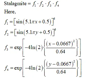
function [f] = stalagmite(input_vector)

x = input_vector(1);
y = input_vector(2);
f1 = (sin(5.1*pi*x+0.5))^6;
f2 = (sin(5.1*pi*y+0.5))^6;
f3 = exp(-4*log(2)*(x-0.0667)^2/0.64);
f4 = exp(-4*log(2)*(y-0.0667)^2/0.64);

f = (f1*f2*f3*f4);
end
FINAL CODE:
FOR GLOBAL MAXIMA:
clear all
close all
clc

%Defining our search space
x = linspace(0,0.6,150);
y = linspace(0,0.6,150);

%creating a two dimensional mesh
[xx yy] = meshgrid(x,y);

%evaluating the stalagmite function
for i = 1:length(xx);
    for j = 1:length(yy);
        input_vector(1) = xx(i,j);
        input_vector(2) = yy(i,j);
         f(i,j) = stalagmite(input_vector);
    end
end
surfc(xx,yy,f)
shading interp
[inputs,fval] = ga(@stalagmite,2)- Writing the Programme with Three Different Optimization Studies:
- In the main program,We are going to make three different studies(one by one) to optimize the solution.
- We use the num_cases = 50 which runs the genetic algorithm 50 times.
- f = get_stalagmite(x,y); is a function whcih helps to genrate stalagmite function.
- We are going to do each study seperately as follows.
FUNCTION:
function f = get_stalagmite(x,y)
for i = 1:length(x)
    for j = 1:length(y)
        f1 = (sin(5.1*pi.*x(i)+0.5)).^6;
        f2 = (sin(5.1*pi.*y(j)+0.5)).^6;
        f3 = exp(-4*log(2).*(x(i)-0.0667).^2/0.64);
        f4 = exp(-4*log(2).*(y(j)-0.0667).^2/0.64);
        f(i,j) = -(f1.*f2.*f3.*f4)
    end
end
end
Study 1:
- In this we are just calling the ga function and passing a number of variables as an input which is equal to 2 and storing the x and y value also the (fopt)optimum value which function is produced.
- tic and study_time toc are used to caluculate the time taken to meausre how long it took.
clear all
close all
clc

x = linspace(0,0.8,150);
y = linspace(0,0.8,150);
num_cases = 50;
f = get_stalagmite(x,y);

tic
for i = 1:num_cases
    [inputs, fopt(i)] = ga(@stalagmite,2);
    xopt(i) = inputs(1);
    yopt(i) = inputs(2);

end
study_time = toc;
- After that opening an new figyre and creating subplot for the two plot windows in the same figure.
- The first plot is surfc(x,y,z) and using plot3 command for x,y and optimum value value of ga predicts over the 50 studies .which helps us to know how the algorithm is performing.
- Now the second subplot in which direct optimum values are getting plotted.
study_time = toc;
figure(1)
fopt = -fopt
subplot(2,1,1)
hold on
surfc(x,y,f)
shading interp
hold on
plot3(xopt,yopt,-fopt,'marker','o','markerfacecolor','r','markersize',5)
title('unbounded inputs')
subplot(2,1,2)
hold on
plot(-fopt)
xlabel('iterations')
ylabel('f minimum')
OUTPUT:
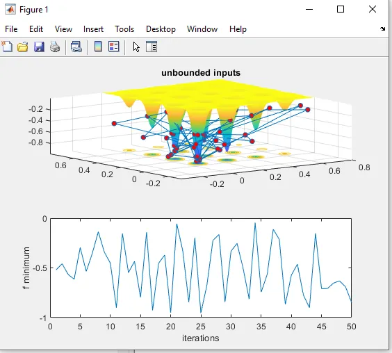
- Due to random sampling and maximum value changes from between 0.2 to 0.8,also time is taken to study is 7.6273
- Further optimization is required
STUDY 2:
- In this both upper and lower bounds are used the syntax used is based on our reffered syntax section.
- Where [0;0] are the upper and lower limit of x
- [1;1] are the upper and lower limit of y
tic
%study for case 2  with upper and lower bounds
for i = 1:num_cases
    [inputs,fopt(i)] = ga(@stalagmite,2,[],[],[],[],[0;0],[1;1]);
    xopt(i) = inputs(1)
    yopt(j) = inputs(2)
end
start_time = toc;
figure(2)
fopt = -fopt
subplot(2,1,1)
surfc(x,y,f)
shading interp
hold on
plot3(xopt,yopt,-fopt,'marker','o','markerfacecolor','r','markersize',5)
title('unbounded inputs')
subplot(2,1,2)
hold on
plot(-fopt)
xlabel('iterations')
ylabel('f minimum')
OUTPUT FOR STUDY 2:
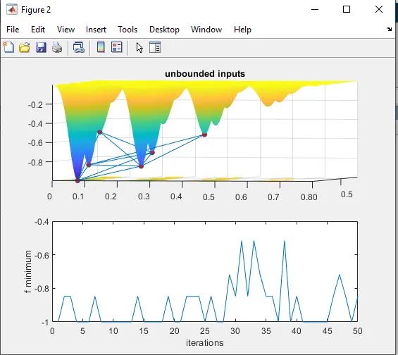
- Here we can see more clear results than the first one.
- Here maximum value is between 0.7 to 0.825 which is much less range.also the time taken is to second study is 10.332 seconds
- Still,Optimization is required further.
STUDY 3:
- To optimize the results and get more accuracy we are increasing the iteration in genetic algorithm.because by default the ga takes 50 value. Here we are going to increase the population size because if population is too small then it is not going to find out global maxima it only fibds local minima.
- Here we are increasing the population size to 170
tic
%study with case 3
%increasing GA iterations
options = optimoptions('ga')
options = optimoptions(options,'populationsize',170)
for i = 1:num_cases
    [inputs,fopt(i)] = ga(@stalagmite,2,[],[],[],[],[0;0],[0.5;0.5],[],[],options)
    xopt(i) = inputs(1)
    yopt(j) = inputs(2)
end
fopt = -fopt
study_time = toc
figure(3)
subplot(2,1,1)
hold on
surfc(x,y,f)
shading interp
title('unbounded inputs')
plot3(xopt,yopt,-fopt,'marker','o','markerfacecolor','r','markersize',5)
subplot(2,1,2)
plot(fopt)
xlabel('iterations')
ylabel('f minimum')
OUTPUT:
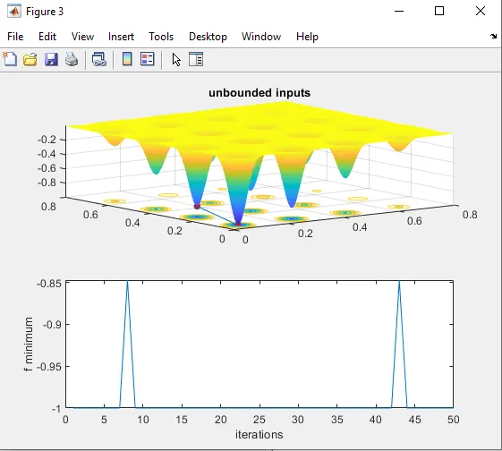
- Here we can see the most accurate result can be seen and hence it is the best result.
FINAL CODES FOR BOTH MAXIMA AND MINIMA:
clear all
close all
clc

%Defining our search space
x = linspace(0,0.6,150);
y = linspace(0,0.6,150);

%creating a two dimensional mesh
[xx yy] = meshgrid(x,y);

%evaluating the stalagmite function
for i = 1:length(xx);
    for j = 1:length(yy);
        input_vector(1) = xx(i,j);
        input_vector(2) = yy(i,j);
         f(i,j) = stalagmite(input_vector);
    end
end
surfc(xx,yy,f)
shading interp
[inputs,fval] = ga(@stalagmite,2)
clear all
close all
clc
x = linspace(0,0.8,150);
y = linspace(0,0.8,150);
num_cases = 50;
f = get_stalagmite(x,y);
tic
for i = 1:num_cases
[inputs, fopt(i)] = ga(@stalagmite,2);
xopt(i) = inputs(1);
yopt(i) = inputs(2);
end
study_time = toc;
figure(1)
fopt = -fopt
subplot(2,1,1)
hold on
surfc(x,y,f)
shading interp
hold on
plot3(xopt,yopt,-fopt,'marker','o','markerfacecolor','r','markersize',5)
title('unbounded inputs')
subplot(2,1,2)
hold on
plot(-fopt)
xlabel('iterations')
ylabel('f minimum')
tic
%study for case 2 with upper and lower bounds
for i = 1:num_cases
[inputs,fopt(i)] = ga(@stalagmite,2,[],[],[],[],[0;0],[1;1]);
xopt(i) = inputs(1)
yopt(j) = inputs(2)
end
start_time = toc;
figure(2)
fopt = -fopt
subplot(2,1,1)
surfc(x,y,f)
shading interp
hold on
plot3(xopt,yopt,-fopt,'marker','o','markerfacecolor','r','markersize',5)
title('unbounded inputs')
subplot(2,1,2)
hold on
plot(-fopt)
xlabel('iterations')
ylabel('f minimum')
tic
%study with case 3
%increasing GA iterations
options = optimoptions('ga')
options = optimoptions(options,'populationsize',170)
for i = 1:num_cases
[inputs,fopt(i)] = ga(@stalagmite,2,[],[],[],[],[0;0],[0.5;0.5],[],[],options)
xopt(i) = inputs(1)
yopt(j) = inputs(2)
end
fopt = -fopt
study_time = toc
figure(3)
subplot(2,1,1)
hold on
surfc(x,y,f)
shading interp
title('unbounded inputs')
plot3(xopt,yopt,-fopt,'marker','o','markerfacecolor','r','markersize',5)
subplot(2,1,2)
plot(fopt)
xlabel('iterations')
ylabel('f minimum')
RESULTS AND CONCLUSION:
- Hence, The MATLAB programe for optimizing the stalagmite function is done
- The graphs for all three studies and global maxima are plotted.