Conjugate Heat Transfer Analysis (CHT) :-

The Conjugate Heat Transfer (CHT) analysis type of CFD analysis, which perform the simulation of heat transfer between solid and fluid domains by exchanging thermal energy at the interfaces between them. In certain critical applications where working temperature is very high, it is necessary to calculate the temperature distribution in the solid to ensure that it should not cross the metallurgical limit. The Selection of the material and wall thickness is largely dependant on the wall temperature distribution in the solid. Hence, it is necessary to solve the energy equation of the solid alongwith the fluid flow equations, commonly known as conjugate heat transfer problem. The important parameters, that are to be analyzed for the successful design of any heat transfer devices are temperature, heatflux and heat transfer coefficient of the surfaces exposed to heating or cooling environment. However accurate calculation of convective heat transfer coefficient requires boundary condition consists of the coupling of solid and fluid fields. Such a boundary condition assumes that the heat convected in or out to or from the solid is absorbed from or rejected to the fluid passing over the solid surface. This situation is highly complex to analyze theoretically since the wall and freestream parameters vary time to time. So, analytical solution for the simplest case of this heat transfer problem necessitates lot of simplified assumptions. Conventionally the solution for the problem has been sought explicitly for fluid and solid.

Conjugate heat transfer problems can be solved by either analytical methods or by numerical methods. The analytical CHT studies require thourough understanding of the given heat transfer problem and involves complex mathematics. Such studies involve lot of simplifications based on certain valid assumptions. Hence the correctness of the solution depends largely on the validity of assumptions made. On the other hand numerical CHT solution methods are relatively simpler if the numerical methods to be followed is clear. Moreover, a correctly implemented numerical CHT solver is not just limited to one CHT problem. Hence the same CHT alogirithm can be applied to several CHT problems with minimum efforts in terms of solution domain modifications.

Using CHT Analysis We can obtain following Parameters:-

1.Internal Combustion Engines

2. Electromobility (Lithium-ion Battry cooling)

3. Heat exchangers

4.Pumps and Compressors

5. Hypersonic aerospace applications

Value of Y+ :-

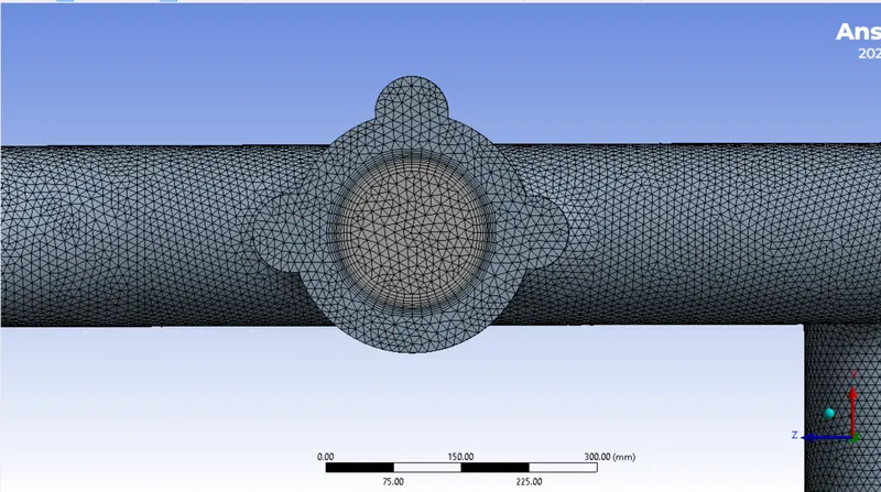
The Y+ values is maintained below 10mm, as the heat transfer coefficient is wall phenomenon, Inflation layers are created by assigning the valu of first layer thickness of 0.4 mm to the interference layer between solid and fluid domain. 'K-epsilon' turbulence model is used for this CHT analysis.

Exhaust-Port CHT Analysis:-

Solid Geometry:-

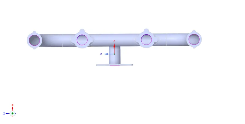
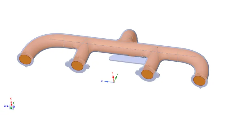
Extracted Fluid Volume and solid Geometry:-

Boundary Conditions:-

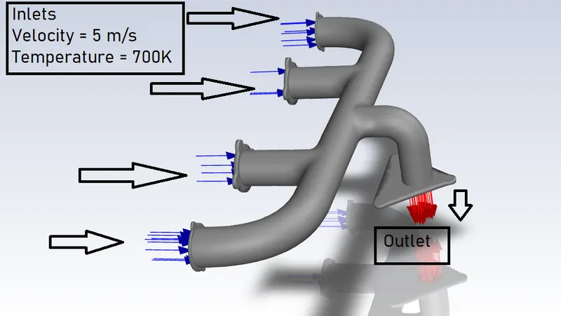
Inlet :-

Inlet Temperature = 700k

velocity = 5 m/s^2

Outlet :-

Pressure-outlet

Pipe wall :-

Convection = 20 W/(m^2 K)

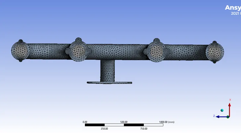
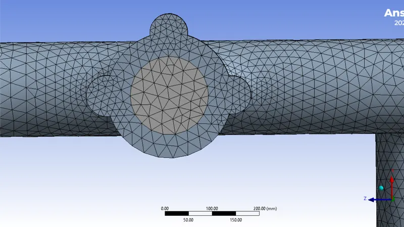
Case 1:- Base Mesh

Mesh Generated:-

Results:-

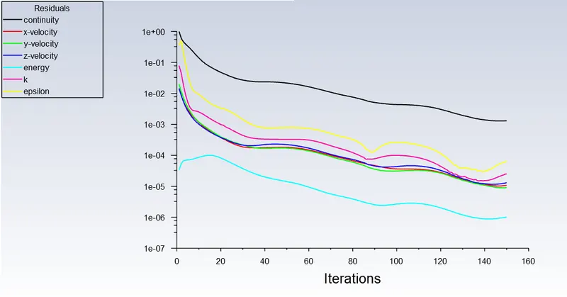
Residuals:-

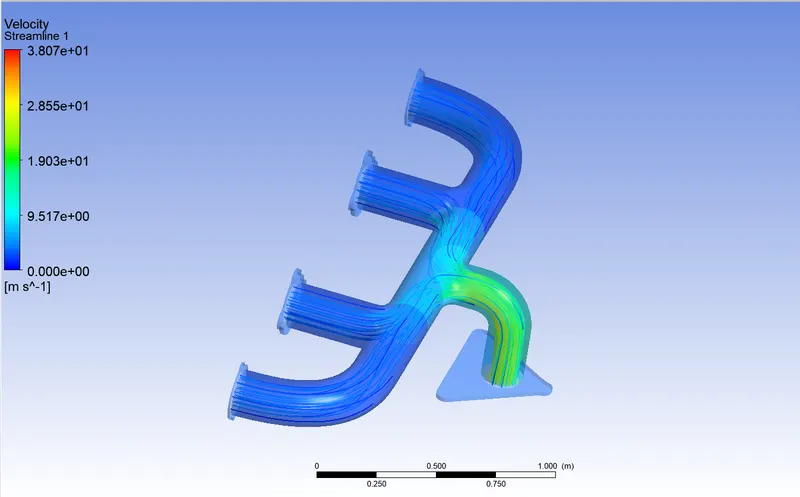
Velocity Streamline :-

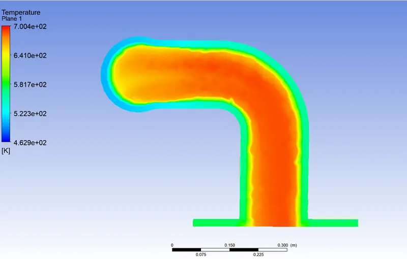
Temperature Contour:-

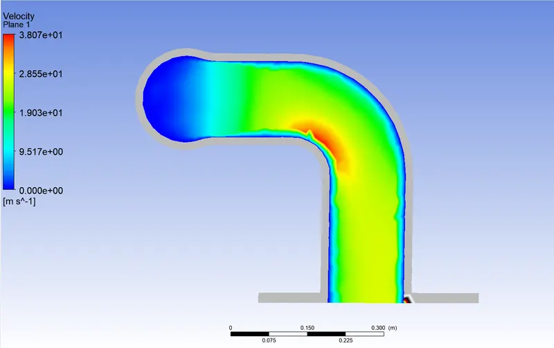
Velocity Contour :-

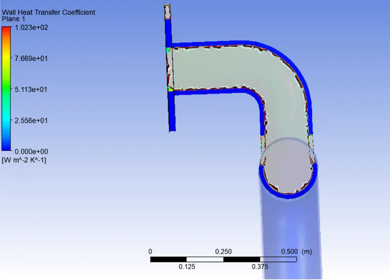
Wall Heat Transfer Coefficent:-

Case 2:- Refined Mesh

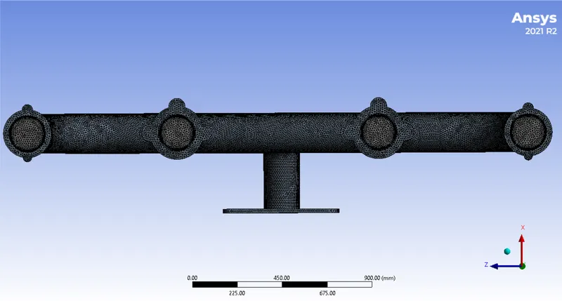
Mesh Generated:-

Results:-

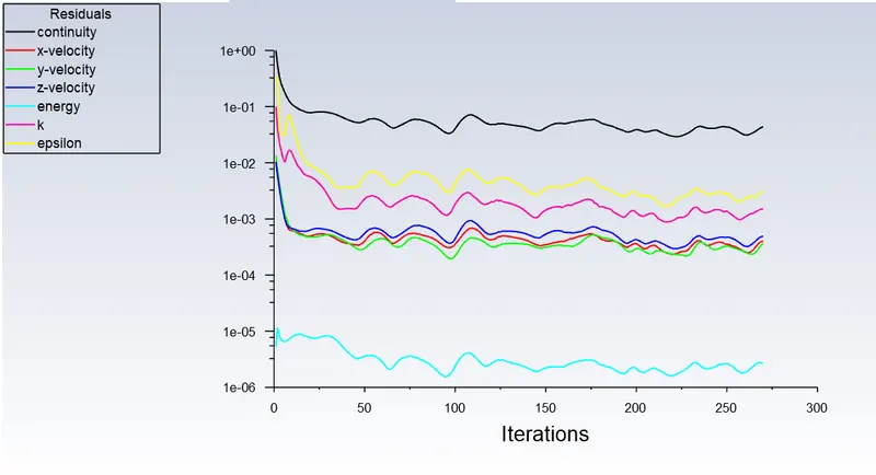
Residuals:-

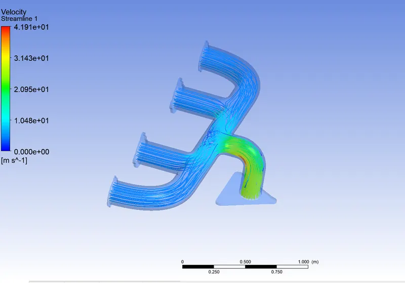
Velocity Streamline :-

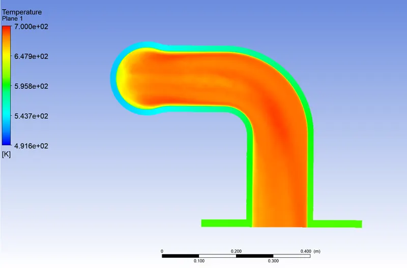
Temperature Contour:-

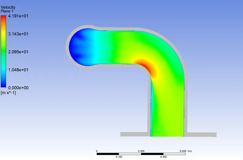
Velocity Contour :-

Wall Heat Transfer Coefficent:-

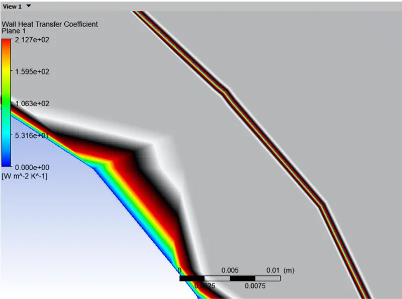
Validation of Results:-

Through experimental methods, we can determine the temperature difference and hence the heat loss or gain through the system. The Nusselt number can be calculated from this data which leads to the calculation of the heat transfer coefficient. There are various empirical relations that can help to calculate Nusselt number analytically. The widely used correlations for flow in a pipe are the Gnielinski correlation and the Dittus-Boelter equation. The Dittus-Bolter equation can be used to calculate the Nusselt number from the Reynold’s number and Prandtl number of the flow.

The factors on which the heat transfer coefficient depends are geometry, the temperature of the flowing fluid in the region, fluid to wall temperature ratio, the inlet velocity of fluid flowing, and also thermal properties of the fluid such as a heat capacity, viscosity, etc. Hence care should be taken in specifying above parameters when solving for heat transfer coefficients.