Week 7 - Simulation of a 1D Super-sonic nozzle flow simulation using Macormack Method
Simulation of 1D supersonic nozzle flow using McCormack’s Method
Objective: -
1.Simulation of 1D supersonic nozzle flow using McCormack’s Method.
- To plot variation in flow field variables in both Non-Conservative form and Conservative form.
3.To compare mass flow rate between both Non-Conservative form and Conservative form.
Nozzle Profile: -
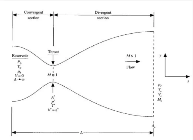
Length = 3m.
A = 1 + 2.2*(x-1.5).^2;
1D mesh along x-axis of nozzle:-
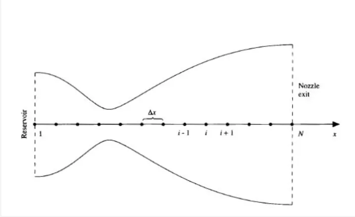
No. of grid points = 61
Non-Conservative Form : -
Non- Conservative form Governing equation:-
Contunity Equation :-
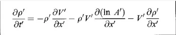
Momentum Equation:-
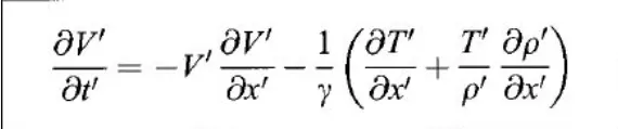
Energy Equation:-

Conservative Form: -
Conservative form Governing equation:-
Continuity Equation:-
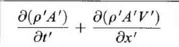
Momentum Equation:-

Energy Equation:-

Steps in McCormack’s Method: -
- Predictor step (using forward differencing)
2.Solution update
- Corrector step (using backward differencing)
4.Taking the average of the time derivative
- Final solution update
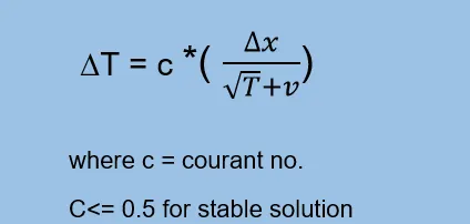
The time step used in the simulation is
Matlab program for the function of Non-Conservative form: -
% Defining matlb function for Non-Conservative form
function [rho,T,v,iteration_no,net_mfr,mach_no,mfr] = Non_Conservation(n,x,dx,c,nt,gamma)

% Defining intial profile
rho = 1-0.3146*x;
T   = 1-0.2314*x;
v   = (0.1 + 1.09*x).*T.^0.5;
a   = 1 + 2.2*(x-1.5).^2;
throat = (n-1)/2;
p = rho.*T;


% Preallocating variables for predictior and corector steps
drhodt_p = zeros(n);
dvdt_p   = zeros(n);
dTdt_p   = zeros(n);

drhodt_c = zeros(n);
dvdt_c   = zeros(n);
dTdt_c   = zeros(n);

net_mfr = zeros(1,nt);

error_rho = 1e9;
error_v   = 1e9;
error_T   = 1e9;

% iteration counter
iteration_no = 0;

 for l = 1:nt

      % Calculating time steps
     dt = min(c.*(dx./(((T.^0.5) + v))));

      % Defining error value for convergence
        error_tolerence = 1e-6;

       % storing intial values
         rho_old = rho;
         T_old   = T;
         v_old   = v;

         % Defining pressure value
            p = rho.*T;

           rho_t(l)     = rho(throat);
           v_t(l)       = v(throat);
           T_t(l)       = T(throat);
           p_t(l)       = p(throat);


   figure(1)
   subplot(4,1,1)
   plot(1:l,rho_t);
   grid on
   xlabel('Timesteps');
   ylabel('Non-dimensional Density');
   title( 'Density');

   subplot(4,1,2)
   plot(1:l,v_t);
   grid on
   xlabel('Timesteps');
   ylabel('Non-dimensional Velocity');
   title( 'Velocity');

   subplot(4,1,3)
   plot(1:l,T_t);
   grid on
   xlabel('Timesteps');
   ylabel('Non-dimensional Temperature');
   title( 'Temperature');

   subplot(4,1,4)
   plot(1:l,p_t);
   grid on
   xlabel('Timesteps');
   ylabel('Non-dimensional Pressure');
   title( 'Pressure');
   sgtitle('Comparison of flow feild varables in non conservative form ');


   if ( error_v > error_tolerence && error_rho > error_tolerence && error_T > error_tolerence)

      % Using Predictor step
   for j = 2:n-1

         % Defining terms to simplify equations
         dvdx      = (v(j+1) - v(j))/dx;
         d_loga_dx = (log(a(j+1)) - log(a(j)))/dx;
         drho_dx   = (rho(j+1) - rho(j))/dx;
         dTdx      = (T(j+1) -T(j))/dx;

         % Using forward differencing approach

         % Defining continuity equation non conservative form
         drhodt_p(j) = -rho(j)*dvdx - rho(j)*v(j)*d_loga_dx - v(j)*drho_dx;

         % Defining Momentum equation non conservative form
         dvdt_p(j)   =  -v(j)*dvdx - (1/gamma)*(dTdx + (T(j)/rho(j))*drho_dx);

         % Defining Energy equation non conservative form
          dTdt_p(j)  =  -v(j)*dTdx - (gamma - 1)*T(j)*(dvdx + v(j)*d_loga_dx);

         % updating solution
          rho(j) = rho_old(j) + drhodt_p(j)*dt;
          v(j)   = v_old(j) + dvdt_p(j)*dt;
          T(j)   = T_old(j) + dTdt_p(j)*dt;
   end

         % Using Corrector step

       for z = 2:n-1

        % Defining terms to simplify equations
         dvdx      = (v(z) - v(z-1))/dx;
         d_loga_dx = (log(a(z)) - log(a(z-1)))/dx;
         drho_dx   = (rho(z) - rho(z-1))/dx;
         dTdx      = (T(z) - T(z-1))/dx;

         % Using backward differencing approach

          % Defining continuity equation non conservative form
         drhodt_c(z) = -rho(z)*dvdx - rho(z)*v(z)*d_loga_dx - v(z)*drho_dx;

         % Defining Momentum equation non conservative form
         dvdt_c(z)   =  -v(z)*dvdx - (1/gamma)*(dTdx + (T(z)/rho(z))*drho_dx);

         % Defining Energy equation non conservative form
          dTdt_c(z)  =  -v(z)*dTdx - (gamma - 1)*T(z)*(dvdx + v(z)*d_loga_dx);

      end

     % Calculating average values

     drhodt = 0.5*(drhodt_p + drhodt_c);
     dvdt   = 0.5*(dvdt_p + dvdt_c);
     dTdt   = 0.5*(dTdt_p + dTdt_c );

     % Solution update
      for i = 2:n-1

         rho(i) = rho_old(i) + drhodt(i)*dt;
         v(i)   = v_old(i) + dvdt(i)*dt;
         T(i)   = T_old(i) + dTdt(i)*dt;

      end

        % Defining boundary conditions
        % at inlet
        v(1) = 2*v(2) - v(3);

        % at outlet
        rho(n) = 2*rho(n-1) - rho(n-2);
        v(n)   = 2*v(n-1) - v(n-2);
        T(n)   = 2*T(n-1) - T(n-2);

      % Calculating Mach no.
      mach_no = v./sqrt(T);

      % Calculating mass flow rate at inlet and outlet
      mfr_inflow  = rho(1)*a(1)*v(1);
      mfr_outflow = rho(n)*a(n)*v(n);

      % Calcutaing net mass flow rate
      net_mfr(l) = mfr_outflow - mfr_inflow;

      error_rho = max(abs(rho - rho_old));
      error_v   = max(abs(v - v_old));
      error_T   = max(abs(T - T_old));

      iteration_no = iteration_no +1;

  end

 end
      % Calculating mass floe rate at different engths
         mfr  = rho.*v.*a;
 end
Matlab program for the function of Conservative form: -
% Defining matlb function for Conservative form
function [rho_c,v_c,T_c,iteration_no_c,net_mfr_c,mach_no_c,mfr_c] = conservation (n,x,dx,nt,gamma,c)

% Defining intial profile
 for i = 1:n

  if (x(i)>=0) && (x(i)<=0.5)
        rho_c(i) = 1;
        T_c(i)   = 1;
     elseif (x(i)>=0.5) && (x(i)<=1.5)
        rho_c(i) = 1 - 0.366*(x(i)-0.5);
        T_c(i)   = 1 - 0.167*(x(i)-0.5);
     elseif (x(i)>=1.5) && (x(i)<=3.2)
        rho_c(i) = 0.634 - 0.3879*(x(i)-1.5);
        T_c(i)   = 0.833 - 0.3507*(x(i)-1.5);

  end

 end

         % Defining aera and velocity
          a_c = 1 + 2.2.*((x-1.5).^2);
          v_c = 0.59./(rho_c.*a_c);
          throat_c = (n-1)/2;

        % Calculating time steps

        dt = min(c.*(dx./(((T_c.^0.5) + v_c))));


u1 = rho_c.*a_c;
u2 = rho_c.*a_c.*v_c;
u3 = rho_c.*(T_c/(gamma-1)+(gamma/2)*(v_c.^2)).*a_c;


% Preallocating variables for predictior and corector steps
du1dt_p   = zeros(1,n);
du2dt_p   = zeros(1,n);
du3dt_p   = zeros(1,n);

j1 = zeros(1,n);
j2 = zeros(1,n);

du1dt_c   = zeros(1,n);
du2dt_c   = zeros(1,n);
du3dt_c   = zeros(1,n);

net_mfr_c = zeros(1,nt);

error_rho = 1e9;
error_v   = 1e9;
error_T   = 1e9;

% iteration counter
iteration_no_c = 0;

% Defining time loop
for  k = 1:nt

     % Defining error value for convergence
       error_tolerence = 1e-5;

      % storing intial values
       u1_old = u1;
       u2_old = u2;
       u3_old = u3;

     % Calculating key variables
       rho_c_old = rho_c;
       T_c_old   = T_c;
       v_c_old   = v_c;

      % Defining pressure value
       p_c = rho_c.*T_c;


   f1 = u2;
   f2 = ((u2.^2)./u1) + ((gamma-1)/gamma)*(u3-((gamma/2)*(u2.^2))./(u1));
   f3 = gamma.*((u2.*u3)./u1) - ((gamma*(gamma-1)/2).*((u2.^3)./u1.^2));

if ( error_v > error_tolerence && error_rho > error_tolerence && error_T > error_tolerence)

    for i = 2:n-1

        j1(i) =  (1/gamma)*rho_c(i)*T_c(i)*(a_c(i+1)-a_c(i))/dx;

    end

     % Using Predictor step
   for j = 2:n-1

     % Defining continuity equation conservative form
       du1dt_p(j) = -(f1(j+1) - f1(j))/dx;

     % Defining Momentum equation conservative form
       du2dt_p(j) = -(f2(j+1) - f2(j))/dx + j1(j);

     % Defining Energy equation conservative form
       du3dt_p(j) = -(f3(j+1) - f3(j))/dx;

       % updating solution
       u1(j) = u1_old(j) +du1dt_p(j)*dt;
       u2(j) = u2_old(j) +du2dt_p(j)*dt;
       u3(j) = u3_old(j) +du3dt_p(j)*dt;

   end


     % Calculating key Variables
      rho_c = u1./a_c;
      v_c = u2./(rho_c.*a_c);
      T_c = (gamma-1)*((u3./u1)-(gamma/2)*v_c.^2);


      f1 = u2;
      f2 = ((u2.^2)./u1) + ((gamma-1)/gamma)*(u3 - ((gamma/2)*(u2.^2)./u1));
      f3 = gamma.*((u2.*u3)./u1) - ((gamma*(gamma-1)/2).*((u2.^3)./u1.^2));

   for i = 2:n-1
       j2(i) = (1/gamma).*rho_c(i)*T_c(i)*(a_c(i) - a_c(i-1))/dx;

   end

   % Using Corrector step

       for j = 2:n-1

         % Defining continuity equation conservative form
          du1dt_c(j) = -(f1(j) - f1(j-1))/dx;

         % Defining Momentum eqcation conservative form
          du2dt_c(j) = -(f2(j) - f2(j-1))/dx + j2(j);

         % Defining Energy equation conservative form
          du3dt_c(j) = -(f3(j) - f3(j-1))/dx;

       end


      % Calculating avarage values
      du1dt_avg = 0.5*(du1dt_p + du1dt_c);
      du2dt_avg = 0.5*(du2dt_p + du2dt_c);
      du3dt_avg = 0.5*(du3dt_p + du3dt_c);

    % Solution update
      for i = 2:n-1

         u1(i) = u1_old(i) + du1dt_avg(i)*dt;
         u2(i) = u2_old(i) + du2dt_avg(i)*dt;
         u3(i) = u3_old(i) + du3dt_avg(i)*dt;

      end


    % Defining boundary conditions
    % at inlet
      u2(1) = 2*u2(2) - u2(3);

     % at outlet
      u1(n) = 2*u1(n-1) - u1(n-2);
      u2(n) = 2*u2(n-1) - u2(n-2);
      u3(n) = 2*u3(n-1) - u3(n-2);

      % Defining key variables
      rho_c = u1./a_c;
      v_c = u2./(rho_c.*a_c);
      T_c = (gamma-1)*((u3./u1) - (gamma/2)*v_c.^2);

      % Calculating Mach no.
      mach_no_c = v_c./sqrt(T_c);

    % Calculating mass flow rate at inlet and outlet
      mfr_inflow  = rho_c(1)*v_c(1)*a_c(1);
      mfr_outflow = rho_c(n)*v_c(n)*a_c(n);

      % Calcutaing net mass flow rate
      net_mfr_c(k) = mfr_inflow - mfr_outflow;

      error_rho = max(abs(rho_c - rho_c_old));
      error_v   = max(abs(v_c - v_c_old));
      error_T   = max(abs(T_c - T_c_old));

      iteration_no_c = iteration_no_c + 1;

end
     % Mass flow rate at different lengths
      mfr_c = rho_c.*v_c.*a_c;

      rho_t_c(k) = rho_c(throat_c);
      v_t_c(k) = v_c(throat_c);
      T_t_c(k) = T_c(throat_c);
      p_t_c(k) = p_c(throat_c);


   figure(2)
   subplot(4,1,1)
   plot(1:k,rho_t_c);
   grid on
   xlabel('Timesteps');
   ylabel('Non-dimensional Density');
   title( 'Density');

   subplot(4,1,2)
   plot(1:k,v_t_c);
   grid on
   xlabel('Timesteps');
   ylabel('Non-dimensional Velocity');
   title( 'Velocity');

   subplot(4,1,3)
   plot(1:k,T_t_c);
   grid on
   xlabel('Timesteps');
   ylabel('Non-dimensional Temperature');
   title( 'Temperature');

   subplot(4,1,4)
   plot(1:k,p_t_c);
   grid on
   xlabel('Timesteps');
   ylabel('Non-dimensional Pressure');
   title( 'Pressure');
    sgtitle('Comparison of flow feild varables in conservative form');

end
Main Matlab program: -
clear all
close all
clc

% Defining no  of grids and other parameters
 n = 61;
 x = linspace(0,3,n);
 dx = x(2) - x(1);

 % Defining courant number
 c =0.5;
 % Defining thermal diffusivity
 %alpha = 1;

 % Defining time step size
 %dt = (c*(dx)^2)/alpha;
  nt    = 1400;
  gamma = 1.4;


 % Calling Non-Conservative form function
  tic
  [rho,T,v,iteration_no,net_mfr,mach_no,mfr] = Non_Conservation(n,x,dx,c,nt,gamma);
  non_conservation_time =toc;

  % Calling Conservative form function
  tic
  [rho_c,v_c,T_c,iteration_no_c,net_mfr_c,mach_no_c,mfr_c] = conservation (n,x,dx,nt,gamma,c);
  conservation_time =toc;


  % Plotting Mass flow rate graphs
  figure(3)
  subplot(2,1,1)
  plot(net_mfr);
  ylim([-1.5 1.5]);
  grid on
  xlabel('No. of timesteps');
  ylabel('Net mass floe rate');
  title('Non Conservative form');

  subplot(2,1,2)
  plot(net_mfr_c);
  ylim([-1.5 1.5]);
  grid on
  xlabel('No. of timesteps');
  ylabel('Net mass floe rate');
  title('Conservative form');


  % Plotting Comparison of flow feild varables in non conservative form and conservative form
  figure(4)
  subplot(4,1,1)
  plot(x,rho,'r');
  hold on
  plot(x,rho_c,'b');
  grid on
  xlabel('Non-dimensional length of nozzle');
  ylabel('Non-dimensional Density');
  legend('Non conservative form','Conservative form');
  title( 'Density');

  subplot(4,1,2)
  plot(x,v,'r');
  hold on
  plot(x,v_c,'b');
  grid on
  xlabel('Non-dimensional length of nozzle');
  ylabel('Non-dimensional Velocity');
  legend('Non conservative form','Conservative form');
  title( 'Velocity');

  subplot(4,1,3)
  plot(x,T,'r');
  hold on
  plot(x,T_c,'b');
  grid on
  xlabel('Non-dimensional length of nozzle');
  ylabel('Non-dimensional Temperature');
  legend('Non conservative form','Conservative form');
  title( 'Temperature');

  subplot(4,1,4)
  plot(x,mach_no,'r');
  hold on
  plot(x, mach_no_c,'b');
  grid on
  xlabel('Non-dimensional length of nozzle');
  ylabel('Mach No');
  legend('Non conservative form','Conservative form');
  title( 'Mach No.');
  sgtitle('Comparison of flow feild varables in non conservative form and conservative form');


  % Plotting graphs for Non Conservation form
   figure(5)
   subplot(2,2,1)
   plot(x,mach_no);
   grid on
   xlabel('Non-dimensional length of nozzle');
   ylabel('Mach No.');
   title( 'Mach No.');

   subplot(2,2,2)
   plot(x,rho);
   grid on
   xlabel('Non-dimensional length of nozzle');
   ylabel('Non-dimensional Density');
   title( 'Density');

   subplot(2,2,3)
   plot(x,v);
   grid on
   xlabel('Non-dimensional length of nozzle');
   ylabel('Non-dimensional Velocity');
   title( 'Velocity');

   subplot(2,2,4)
   plot(x,T);
   grid on
   xlabel('Non-dimensional length of nozzle');
   ylabel('Non-dimensional Temperature');
   title( 'Temperature');

   sgtitle(sprintf('Quasi 1D Supersonic nozzle flow: Non Conservation form\nNo.of iterations =%d\nTime for convergence = %f s',iteration_no,non_conservation_time));


  % Plotting graphs for Conservation form
   figure(6)
   subplot(2,2,1)
   plot(x,mach_no_c);
   grid on
   xlabel('Non-dimensional length of nozzle');
   ylabel('Mach No.');
   title( 'Mach No.');

   subplot(2,2,2)
   plot(x,rho_c);
   grid on
   xlabel('Non-dimensional length of nozzle');
   ylabel('Non-dimensional Density');
   title( 'Density');

   subplot(2,2,3)
   plot(x,v_c);
   grid on
   xlabel('Non-dimensional length of nozzle');
   ylabel('Non-dimensional Velocity');
   title( 'Velocity');

   subplot(2,2,4)
   plot(x,T_c);
   grid on
   xlabel('Non-dimensional length of nozzle');
   ylabel('Non-dimensional Temperature');
   title( 'Temperature');

  sgtitle(sprintf('Quasi 1D Supersonic nozzle flow: Conservation form\nNo.of iterations =%d\nTime for convergence = %f s',iteration_no_c,conservation_time));
Output Graphs:-
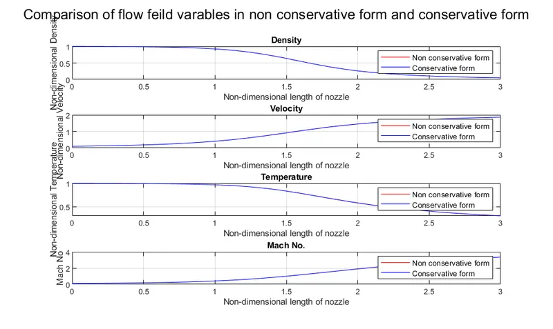
Figure(1): -Comparison of flow field variables in non-conservative form and conservative form
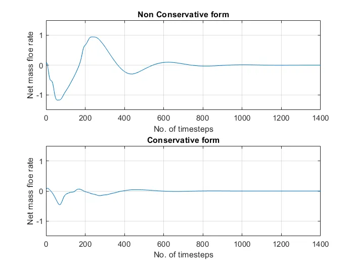
Figure(2): - Comparison of mass flow rate in non-conservative and conservative form
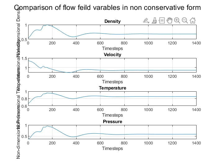
Figure(3): - Variation of flow primitive variables in the non-conservative form
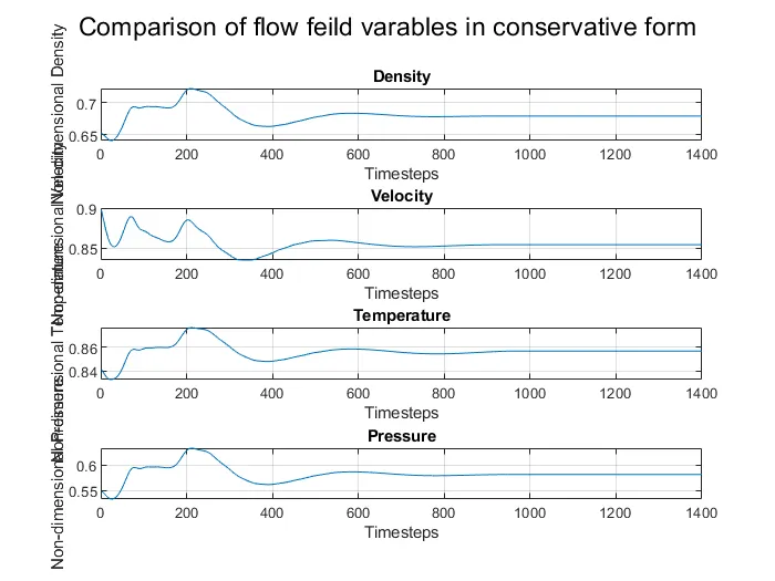
Figure(4): - Variation of flow primitive variables in the conservative form
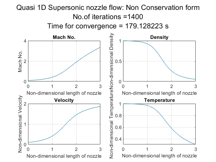
Figure(5): The Non-conservative form Iterations
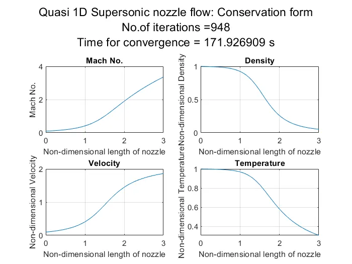
Figure(6): The Conservative form Iterations
Conclusion: -
1.For both Non-conservative form and Conservative form mach no. and velocity increase along the length of nozzle and at throat value of mach no. is equal to 1. Whereas, temperature and density decrease along the length of the nozzle.
2.The net mass flow rate in both the Non-conservative form and Conservative form gets stable around 500 timesteps. However, in the Non-conservative form at the beginning amplitude variation is very high in comparison to the Conservative form.
3.The key flow fields are almost similar in both the Non-conservative form and Conservative form, which proves the reliability of the solution.
4.Increasing grid points more than 31 does not change flow variable value much, beyond 31 grid points flow variable values have minor changes. Hence, at 31 nodes numerical solutions achieve grid independence.