Week 3.5 - Deriving 4th order approximation of a 2nd order derivative using Taylor Table method

Deriving fourth (4^th) order approximations of second-order derivatives

1. Fourth-order approximation of second-order derivative using central differencing, Consider numerical stencil below for central differencing scheme,

The hypothesis equation for CDS is,

`(∂^2 u)/(∂x^2 )` = a∙f (i-2) + b∙f (i-1) + c∙f(i) + d∙f(i+1) + e ∙f(i+2)

Using Taylor’s table to find the values of unknown coefficient,

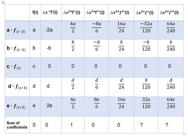
Ignoring the last two columns as we have 5 unknowns and we need 5 equations.

a + b + c +d + e = 0

-2*a - b + d + 2*e = 0

2*a + b/2 + d/2 + 2*e = 1

-(8/6) *a – b/6 + d/6 + (8/6) *e = 0

(16/24) *a +b/24 + d/24 + (16/24) *e = 0

Writing equations in matrix form to solve,

A = [1 1 1 1 1; -2 -1 0 2 1; 2 0.5 0 0.5 2; -8\6 -1\6 0 1\6 8\6; 16\24 1\24 0 1\24 16\24];

B = [ 0;0;1;0;0];

X = linsolve (A, B)

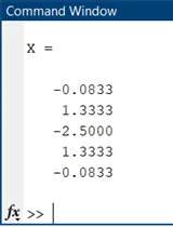
Solving above matrix in Matlab we get coefficient values as below,

a = -0.0833

b = 1.3333

c = -2.5000

d = 1.3333

e =-0.0833

Therefore, a=e and b=d.

Sum of column 1= a + b + c + d + e = 0,

Sum of column 2 = 0

Sum of column 3 = 1

Sum of column 4 = 0

Sum of column 5 = 0

Sum of column 6 = 0

Sum of column 7 = 2* (64*a/720 + b/720), is non zero.

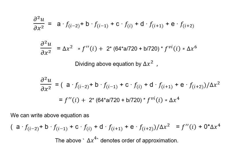
2. Fourth-order approximation of second-order derivative using Skewed right-sided differencing, consider numerical stencil below for Skewed right-sided differencing scheme,

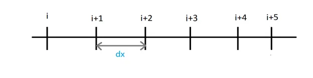
The hypothesis equation is,

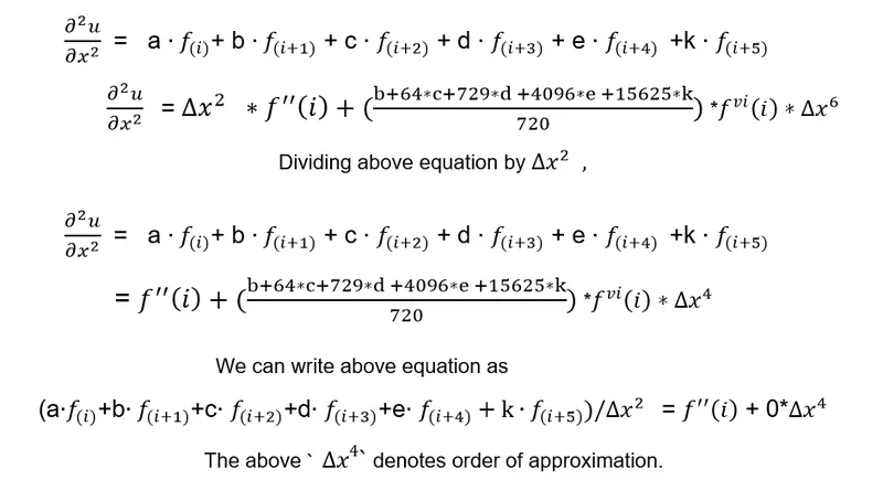
`(∂^2 u)/(∂x^2 )`= a∙f(i)+ b∙f(i+1)+c∙f(i+2)+d∙f(i+3)+e ∙f(i+4)+k∙f(i+5)

Using Taylor’s table to find the values of unknown coefficient,

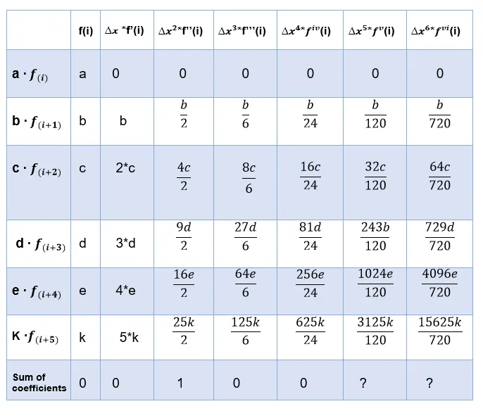
Ignoring last two columns as we have 6 unknowns and we need 6 equations.

a + b + c +d + e + k = 0

0 + b + 2*c +3*d + 4*e + 5*k = 0

0+ b/2 + 4c/2 + 9d/2 + 16e/2 + 25k/2 = 1

0+ b/6 + 8c/6 + 27d/6 + 64e/6 + 125k/6 = 0

0+ b/24 + 16c/24 + 81d/24 + 256e/ 24+ 625k/24= 0

0+ b/120 + 32c/120 + 243d/120 + 1024e/120 + 3125k/120 = 0

Writing equations in matrix form to solve,

C = [ 1 1 1 1 1 1;

0 1 2 3 4 5;

0 1/2 4/2 9/2 16/2 25/2;

0 1/6 8/6 27/6 64/6 125/6;

0 1/24 16/24 81/24 256/24 625/24;

0 1/120 32/120 243/120 1024/120 3125/120];

D = [ 0; 0; 1; 0 ;0; 0];

Y = linsolve (C, D);

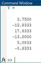
Solving above matrix in Matlab we get coefficient values as below,

a = 3.7500

b = -12.8333

c = 17.8333

d = -13.0000

e = 5.0833

k = -0.8333

Sum of column 1= a + b + c + d + e + k= 0,

Sum of column 2 = 0

Sum of column 3 = 1

Sum of column 4 = 0

Sum of column 5 = 0

Sum of column 6 = 0

Sum of column 7 = (b+ 64*c + 729*d + 4096*e + 15625*k)/720, is non zero.

3. Fourth-order approximation of second-order derivative using Skewed left-sided differencing, consider numerical stencil below for Skewed left-sided differencing scheme,

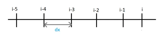
Hypothesis equation is,

`(∂^2 u)/(∂x^2 )` = a ∙f(i-5)+b∙f(i-4)+c∙f(i-3)+d∙f(i-2)+e ∙f(i-1)+k∙f(i)

Using Taylor’s table to find the values of unknown coefficient,

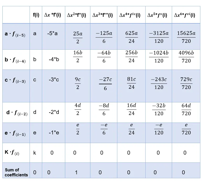
Ignoring last two columns as we have 6 unknowns and we need 6 equations.

a + b + c +d + e + k = 0

(-5*a) – (4 *b) – (3*c) – (2*d) – e + 0 = 0

25a/2 +16b/2 + 9c/2 + 4d/2 + e/2 + 0 = 1

(-125a/6) – (64b/6) – (27c/6) – (8d/6) – (e/6) + 0 = 0

625a/24 + 256b/24 + 81c/24 + 16d/24 + e/24 + 0 = 0

(-3125a/120) – (1024b/120) – (243c/120) – (32d/120) – (e/120) + 0 = 0

Writing equations in matrix form to solve,

E = [ 1 1 1 1 1 1;

-5 -4 -3 -2 -1 0;

25/2 16/2 9/2 4/2 1/2 0;

-125/6 -64/6 -27/6 -8/6 -1/6 0;

625/24 256/24 81/24 16/24 1/24 0;

-3125/120 -1024/120 -243/120 -32/120 -1/120 0];

F = [ 0; 0; 1; 0 ;0 ;0];

Z = linsolve (E, F);

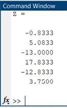
Solving above matrix in Matlab we get coefficient values as below,

a = -0.8333

b = 5.0833

c = -13.0000

d = 17.8333

e = -12.8333

k = 3.7500

Sum of column 1= a + b + c + d + e + k= 0,

Sum of column 2 = 0

Sum of column 3 = 1

Sum of column 4 = 0

Sum of column 5 = 0

Sum of column 6 = 0

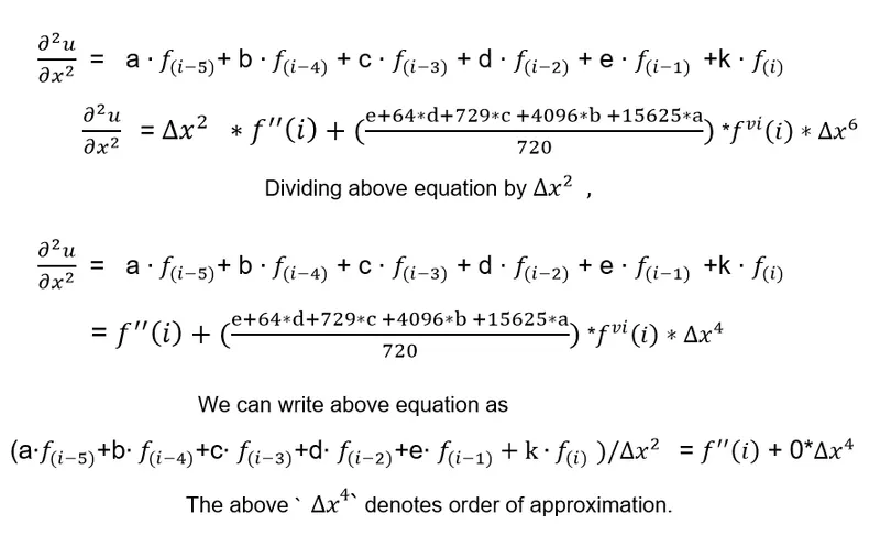
Sum of column 7 = (e+ 64*d + 729*c+ 4096*b + 15625*a)/720, is non zero.

Matlab Program: -

Defining functions :

1. Central differencing function

% Defining function for central differencing scheme
function out = central_differencing_approximation(x,dx)

%f(x)= exp(x)*cos(x)

%defining analytical derivative of a function 

analytical_derivative = -2*exp(x)*sin(x);
% defining Numerical deriviative 
% central differencing = a*f(i-2)+b*f(i-1)+c*f(i)+d*f(i+1)+e*f(i+2)
    a = -0.0833;
    b = 1.3333;	
    c = -2.5000;
    d = 1.3333;
    e =-0.0833;
central_differencing = ((a*exp(x-(2*dx))*cos(x-(2*dx)))+ (b*exp(x-dx)*cos(x-dx))+ (c*exp(x)*cos(x))+(d*exp(x+dx)*cos(x+dx))+(e*exp(x+(2*dx))*cos(x+(2*dx))))/(dx^2);

out = abs(central_differencing - analytical_derivative);
end

2. Right skewed approximation function

% Defining function for right skewed differencing scheme
function out = right_skewed_approximation(x,dx)

%f(x)= exp(x)*cos(x)

%defining analytical derivative of a function 

analytical_derivative = -2*exp(x)*sin(x);
% defining Numerical deriviative 
% rightskewed differencing = a*f(i)+b*f(i+1)+c*f(i+2)+d*f(i+3)+e*f(i+4)+k*f(i+5)
 a = 3.7500;
 b = -12.8333;
 c = 17.8333;
 d = -13.0000;
 e = 5.0833;
 k = -0.8333;

 right_skewed_approximation = ((a*exp(x)*cos(x))+(b*exp(x+dx)*cos(x+dx))+ (c*exp(x+(2*dx))*cos(x+(2*dx)))+ (d*exp(x+(3*dx))*cos(x+(3*dx)))+(e*exp(x+(4*dx))*cos(x+(4*dx)))+(k*exp(x+(5*dx))*cos(x+(5*dx))))/(dx^2);
 
 out= abs(right_skewed_approximation - analytical_derivative);
end

3. Left skewed approximation function

% Defining function for left skewed differencing scheme
function out = left_skewed_approximation(x,dx)

%f(x)= exp(x)*cos(x)

%defining analytical derivative of a function 

analytical_derivative = -2*exp(x)*sin(x);
% defining Numerical deriviative 
% leftskewed differencing = a*f(i-5)+b*f(i-4)+c*f(i-3)+d*f(i-2)+e*f(i-1)+k*f(i)
   a = -0.8333;
   b = 5.0833;
   c = -13.0000;
   d = 17.8333;
   e = -12.8333;
   k = 3.7500;

 left_skewed_approximation = ((a*exp(x-(5*dx))*cos(x-(5*dx)))+(b*exp(x-(4*dx))*cos(x-(4*dx)))+ (c*exp(x-(3*dx))*cos(x-(3*dx)))+ (d*exp(x-(2*dx))*cos(x-(2*dx)))+(e*exp(x-dx)*cos(x-dx))+(k*exp(x)*cos(x)))/(dx^2);
 
 out= abs(left_skewed_approximation - analytical_derivative);
end

2. Right skewed approximation function

% Forward differencing scheme

function out = forward_approximation(x,dx)

%f(x)= exp(x)*cos(x)
%defining analytical derivative of function 

analytical_derivative = -2*exp(x)*sin(x);

% defining numerical derivative
%forward_differencing = (f(x+dx)-f(x))/(dx)

forward_difference = ((exp(x+dx)*cos(x+dx))-(exp(x)*cos(x)))/(dx);

out = abs(forward_difference - analytical_derivative);
end

2. Backward skewed approximation function

% Backward differencing scheme

function out = backward_approximation(x,dx)

%f(x)= exp(x)*cos(x)
%defining analytical derivative of function 

analytical_derivative = -2*exp(x)*sin(x);

% defining numerical derivative
%backward_differencing = (f(x-dx)-f(x))/(dx)

backward_difference = ((exp(x-dx)*cos(x-dx))-(exp(x)*cos(x)))/(dx);

out = abs(backward_difference - analytical_derivative);
end

Main Matlab Program:-

clear all
close all
clc

%defining value of x and range for dx
x = pi/3;
dx = linspace(pi/4,pi/4000,40);

for i=1:length(dx)
    %calculetting central difference error
central_difference_error(i) = central_differencing_approximation(x,dx(i));

%calculetting right skewed error
right_skewed_error(i) = right_skewed_approximation(x,dx(i));

%calculetting left skewed error
left_skewed_error(i) = left_skewed_approximation(x,dx(i));

%calculetting forward difference error
forward_difference_error(i) = forward_approximation(x,dx(i));

%calculetting backward difference error
backward_difference_error(i) = backward_approximation(x,dx(i));

end

%plotting Graphs
figure(1)
loglog(dx,central_difference_error,'r','linewidth',3);
hold on
loglog(dx,right_skewed_error,'b','linewidth',3);
hold on
loglog(dx,left_skewed_error,'y','linewidth',3);
hold on
xlabel('Values of dx');
ylabel('Absolute error values');
legend('central difference error','right skewed error', 'left skewed error');
title('Comparison of central differencing, skewed right and skewed left approximations');
pause(0.4);
figure(2)
loglog(dx,forward_difference_error,'m','linewidth',3);
hold on
loglog(dx,backward_difference_error,'g','linewidth',3);
xlabel('Values of dx');
ylabel('Absolute error values');
legend('forward difference error', 'backward difference error');

Output Graphs: -

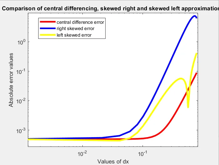
Figure(1): Comparison of central differencing, skewed right and skewed left approximations

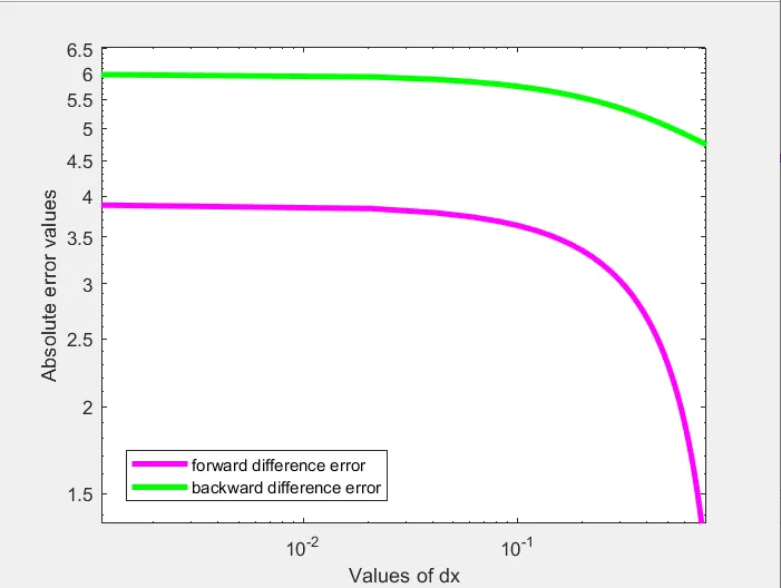
Figure (2): Comparison of forward difference error and backward difference error

Conclusion: -

1. 1. FDS and BDS are first-order approximations with first order derivatives, while CDS solves second-order approximations with first order derivatives, hence CDS is more accurate than FDS and BDS.
2. The central differencing method provides the best results with minimum errors, but it is not useful for the elements near boundaries as we don’t have symmetrical elements on both sides. In such a case, we can obtain better accuracy with minimum error using the Right skewed scheme or Left skewed scheme depending upon the availability of nodes on either side.