Week 5.1 - Mid term project - Solving the steady and unsteady 2D heat conduction problem
1.Steady State Analysis: -
2D Steady-state heat conduction equation is,
`(delta ^2T)/(delta x^2)+(delta ^2T)/(delta y^2) = 0`
using central differencing scheme we get,
T(i,j) = `(Deltax^2Deltay^2) /(2(Deltax^2 + Deltay^2)) * [ (( T(i-1,j) + T(i+1,j))/(Deltax^2))+(( T(i,j-1) + T(i,j+1))/(Deltay^2))]`
Matlab Program:-
clear all
close all
clc
% Defining given parametres
L = 1;
nx = 100;
ny = 100;

x  = linspace(0,L,nx);
dx = x(2)-x(1);
y = linspace(0,L,ny);
dy = y(2)-y (1);

% Defining Temprature conditions
T = 300*ones(ny,nx);
T(:,1) = 400;
T(1,:) = 600;
T(:,end) = 800;
T(end,:) = 900;

T_old = T;

term = (dx^2*dy^2)/(2*(dx^2+dy^2));
tolerence = 1e-4;
error = 1;

% Defining iteration methods
  iteration_method = 3;
%iteration_method = 1-Jacobi, 2-Gauss seidal, 3-SOR
if iteration_method == 1
    tic
    iteration = 0;
    while (error > tolerence)
        for j = 2:ny-1
          for i = 2:nx-1
            T(i,j) = term*((T_old(i-1,j)+T_old(i+1,j))/(dx^2)+(T_old(i,j-1)+T_old(i,j+1))/(dy^2));
         end
        end
        error = max(max(abs(T-T_old)));
        T_old = T;
        iteration = iteration+1;
    end
     time = toc;
elseif iteration_method == 2
    tic
    iteration = 0;
      while (error > tolerence)
         for j = 2:ny-1
          for i = 2:nx-1
            T(i,j) = term*((T(i-1,j)+ T_old(i+1,j))/(dx^2)+(T(i,j-1)+ T_old(i,j+1))/(dy^2));
         end
        end
        error = max(max(abs(T-T_old)));
        T_old = T;
        iteration = iteration+1;
      end
       time = toc;
elseif iteration_method == 3
    omega = 1.8;
    tic
    iteration = 0;
     while (error > tolerence)
        for j = 2:ny-1
         for i = 2:nx-1
            T(i,j) = term*((T(i-1,j)+ T_old(i+1,j))/(dx^2)+(T(i,j-1)+ T_old(i,j+1))/(dy^2));
            T(i,j) = T_old(i,j)*(1-omega)+(omega*T(i,j));
         end
        end
        error = max(max(abs(T-T_old)));
        T_old = T;
        iteration = iteration+1;
     end
      time = toc;
end

% Plotting Temprature contour on X and Y axes
[m,n] = contourf(x,y,T);
clabel(m,n)
colorbar
colormap(jet)
ax = gca;
ax.YDir = 'reverse';
xlabel('X-axis')
ylabel('Y-axis')
title({'steady state temprature contour';['Iteration method = ', num2str(iteration_method)];['No. of Iterations = ',num2str(iteration)];['Simulation Time = ',num2str(time),'s']})
grid on
Output Contour Plots: -
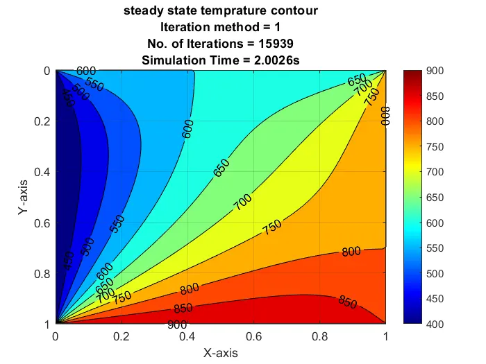
Figure(1): Steady-state temperature contour (Jacobi Method)
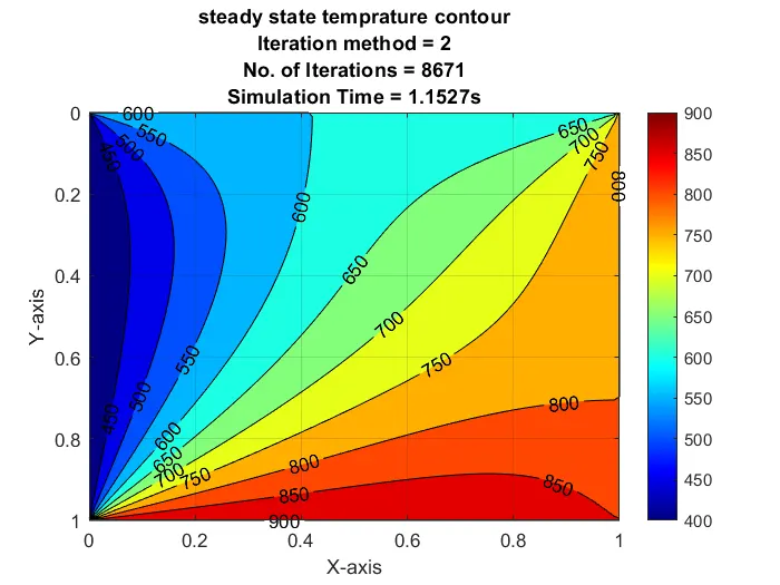
Figure(2): Steady-state temperature contour (Gauss-Seidel Method)
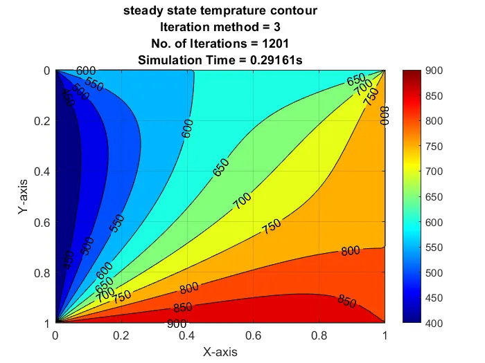
Figure(3): Steady-state temperature contour (SOR Method)
Conclusion: -
SOR method required less no. of iterations and simulation time compared to Gauss seidel and Jacobi. Jacobi method required a large no. of iterations and simulation time than other methods.
2.Transient State Analysis by Explicit Method: -
2D Transient-State heat conduction equation is,
`(delta ^2T)/(delta t^2) = (delta ^2T)/(delta x^2)+(delta ^2T)/(delta y^2)`
Using a forward differencing scheme for time derivative and central differencing scheme for space derivative,
T(i,j) = `T^(n+1)(i,j) = T(i,j)+((alpha Deltat) /(Deltax^2))*[ (( T(i-1,j) - 2T(i,j) + T(i+1,j))]^n+((alpha Deltat) /(Deltay^2))*[(( T(i,j-1) - 2T(i,j)+ T(i,j+1))]^n`
Matlab Program:-
clear all
close all
clc
% Defining given parametres
L = 1;
nx = 100;
ny = 100;
dt = 0.14;
t = 1000;
nt =t/dt;
alpha = 1.75e-4;

x  = linspace(0,L,nx);
dx = x(2)-x(1);
y = linspace(0,L,ny);
dy = y(2)-y (1);

% Calculetting CFL NO.
CFL = alpha*dt*((1/dx^2)+(1/dy^2));

% Defining Temperature conditions
T = 300*ones(ny,nx);
T(:,1) = 400;
T(1,:) = 600;
T(:,end) = 800;
T(end,:) = 900;
T_old = T;

% Defining terms k1 and k2
k1 = (alpha*dt)/(dx^2);
k2 = (alpha*dt)/(dy^2);

% Defining time lop
iteration = 0;
    tic
    for k = 1:nt
        % Defining space loop for X-axis
        for  i = 2:nx-1
        %  Defining space loop for Y-axis
         for j = 2:ny-1
             H = (T_old(i-1,j)-2*T_old(i,j)+T_old(i+1,j));
             V = (T_old(i,j-1)-2*T_old(i,j)+T_old(i,j+1));
             T(i,j) = T_old(i,j)+(H*k1)+(V*k2);
         end
        end
        T_old = T;
        iteration  = iteration+1;
    end
    time =toc;

    % Plotting Temprature contour on X and Y axes
[m,n] = contourf(x,y,T);
clabel(m,n)
colorbar
colormap(jet)
ax = gca;
ax.YDir = 'reverse';
xlabel('X-axis')
ylabel('Y-axis')
title({'Transient state Implicit Method temprature contour';['No. of Iterations = ',num2str(iteration)];['Simulation Time = ',num2str(time),'s'];['CFL = ',num2str(CFL)];['Time = ', num2str(t),'s']})
grid on
Output Contour Plot: -
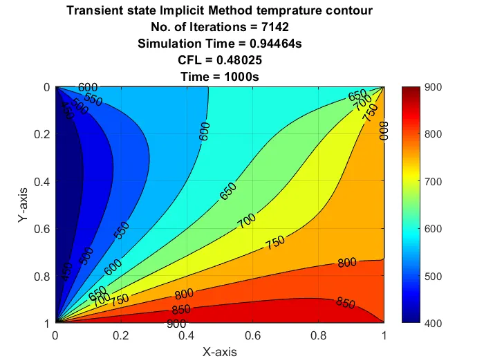
Figure(4): Transient-state temperature contour (Explicit Method)
Temperature contour profile changes with respect to time and then achieves steady-state condition.
3.Transient State Analysis by Implicit Method: -
2D Transient-State heat conduction equation is,
`(delta ^2T)/(delta t^2) = (delta ^2T)/(delta x^2)+(delta ^2T)/(delta y^2)`
Using a forward differencing scheme for time derivative and central differencing scheme for space derivative,
T(i,j) = `T^(n+1)(i,j) = T(i,j)+(alpha Deltat)*[ (( T(i-1,j) - 2T(i,j) + T(i+1,j))/(Deltax^2))+(( T(i,j-1) - 2T(i,j)+ T(i,j+1))/(Deltay^2))]^(n+1)`
Matlab Program:-
clear all
close all
clc
% Defining given parametres
L = 1;
nx = 100;
ny = 100;
dt = 10;
t = 1000;
nt =t/dt;
alpha = 1.75e-4;

x  = linspace(0,L,nx);
dx = x(2)-x(1);
y = linspace(0,L,ny);
dy = y(2)-y (1);

% Calculetting CFL NO.
CFL = alpha*dt*((1/dx^2)+(1/dy^2));

% Defining Temperature conditions
T = 300*ones(ny,nx);
T(:,1) = 400;
T(1,:) = 600;
T(:,end) = 800;
T(end,:) = 900;
T_old = T;
T_prev = T;

% Defining terms k1 and k2
k1 = (alpha*dt)/(dx^2);
k2 = (alpha*dt)/(dy^2);
tolerence = 1e-4;

% Defining iteration methods
  iteration_method = 3;
%iteration_method = 1-Jacobi, 2-Gauss seidal, 3-SOR
if iteration_method == 1
    tic
    iteration = 1;
     for k =1:nt
         error = 1;
    while (error > tolerence)
        for j = 2:ny-1
          for i = 2:nx-1
              term1 = 1/(1+2*k1+2*k2);
              term2 = k1*term1;
              term3 = k2*term1;
              H = (T_old(i-1,j)+T_old(i+1,j));
              V = (T_old(i,j-1)+T_old(i,j+1));
              T(i,j) = (T_prev(i,j)*term1)+(H*term2)+(V*term3);
         end
        end
        error = max(max(abs(T-T_old)));
        T_old = T;
        iteration = iteration+1;
    end
    T_prev =T;
     end
     time = toc;

elseif iteration_method == 2
    tic
    iteration = 1;
    for k =1:nt
    error = 1;
      while (error > tolerence)
         for j = 2:ny-1
          for i = 2:nx-1
              term1 = 1/(1+2*k1+2*k2);
              term2 = k1*term1;
              term3 = k2*term1;
              H = (T(i-1,j)+T_old(i+1,j));
              V = (T(i,j-1)+T_old(i,j+1));
              T(i,j) = (T_prev(i,j)*term1)+(H*term2)+(V*term3);
         end
        end
        error = max(max(abs(T-T_old)));
        T_old = T;
        iteration = iteration+1;
      end
      T_prev = T;
end
       time = toc;

 elseif iteration_method == 3
    omega = 1.1;
    tic
    iteration = 1;
    for k = 1:nt
        error = 1;
     while (error > tolerence)
        for j = 2:ny-1
         for i = 2:nx-1
           term1 = 1/(1+2*k1+2*k2);
              term2 = k1*term1;
              term3 = k2*term1;
              H = (T(i-1,j)+T_old(i+1,j));
              V = (T(i,j-1)+T_old(i,j+1));
              T(i,j) = (T_prev(i,j)*term1)+(H*term2)+(V*term3);
              T(i,j) = T_old(i,j)*(1-omega)+(omega*T(i,j));
         end
        end
        error = max(max(abs(T-T_old)));
        T_old = T;
        iteration = iteration+1;
     end
     T_prev =T;
    end
      time = toc;
end

% Plotting Temprature contour on X and Y axes
[m,n] = contourf(x,y,T);
clabel(m,n)
colorbar
colormap(jet)
ax = gca;
ax.YDir = 'reverse';
xlabel('X-axis')
ylabel('Y-axis')
title({'Transient state Implicit Method temprature contour';['Iteration method = ', num2str(iteration_method)];['No. of Iterations = ',num2str(iteration)];['Simulation Time = ',num2str(time),'s'];['CFL = ',num2str(CFL)];['Time = ', num2str(t),'s']})
grid on
Output Contour Plots: -
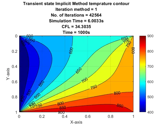
Figure(5): Transient-state temperature contour (Jacobi Method)
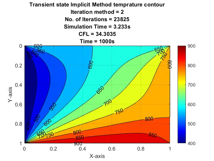
Figure(6): Transient-state temperature contour (Gauss seidal Method)
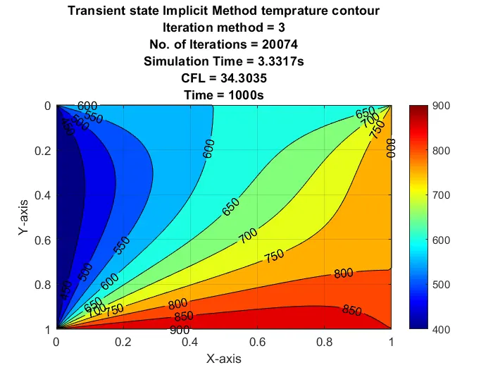
Figure(7): Transient-state temperature contour (SOR Method)
Conclusion: -
1.SOR method required less no. of iterations and simulation time compared to Gauss seidel and Jacobi. Jacobi method required a large no. of iterations and simulation time than other methods.
2.The solution contour obtained is similar to the explicit method.