Week 4 - CHT Analysis on Exhaust port

AIM:

To perform steady-state simulation at an input velocity value of 5m/s to understand the development of the velocity and temperature profiles for the given Exhaust port model and to calculate the wall heat transfer coefficient on the internal solid surface.

OBJECTIVE:

• To understand what is conjugate heat transfer.
• To understand how heat transfer coefficient is calculated for internal flow.
• To study the effect of Reynold's number on the heat transfer coefficients.
• To set-up the convective heat boundary condition for simulation.
• To post process the results form the simulation and validate with the analytical solutions.

INTRODUCTION:

CHT Analysis

• The Conjugate Heat Transfer (CHT) analysis type allows for the simulation of heat transfer between solid and fluid domains by exchanging thermal energy at the interfaces between them.

• Heat transfer rate or coefficient of heat transfer is depending on the Newton's law of cooling which is given by:

`Q=hA(T_1-T_2 )`

Where,

Q is the heat flux (W)

h is heat transfer coefficient (W/m^2K)

A is the surface area where heat transfer takes place (m^2)

T1 is the temperature of the wall (K)

T2 is the temperature of the fluid volume (K)

• The CHT analysis of any given system consider the physical processes and the corresponding governing equation involved for the individual subdomains separately and then correlating their solutions by matching the required condition at the interface to get the distribution of temperature and heat flux in coupled manner thereby eliminating the need of heat transfer coefficient.
• The CHT analysis thus offers advantage of monitoring both fluid and heat transfer changes as well as real time prediction of wall heat transfer coefficient, temperature and velocity profiles across the domain.

Why CHT analysis is used?

• The CHT approach has an advantage over Finite element thermal analyses in that wall heat transfer coefficients and their local variations on surfaces are directly calculated within the model rather than based on simplified empirical calculations. The CHT approach therefore has benefits for those applications where heat transfer is either non-uniform or difficult to calculate empirically.
• The CHT analysis is required to control the cooling rate by predicting the heat transfer coefficient and to show the temperature variation of solid.
• CHT is also used in analyzing the heat transfer in a heat exchanger. A shell and tube heat exchanger is a perfect example of CHT, here one fluid flows throuh tubes and other fluid flows in the shell over the tubes. The heat is transferred from one fluid to the walls of the tube and then from the tube wall to the other fluid in the shell. Here, CHT analysis is useful for predictiing the heat transfer coefficient and to improve the effective heat transfer rate. CHT is also used in analyzing the cooling of electronic devices.

Where CHT analysis is used?

• The application of conjugate heat transfer is varying according to domain. The most important application of this simulations are heat exchangers. In heat exchanger, it is important to lower the temperature of working fluid to get desired result, also its main focus on to lower design material from which fluid is flowing.
• In automobile sector, radiator is a main heat exchanger to lower the fluid temperature which is suppllied to car HVAC system. It uses fins for convection heat transfer between solid and fluid.
• CHT simulations are done in aerospace industry to design suitable material for engine cover. As the temperature generated during the ignition is high enough to melt certian part of engine cover, hence it is important to know how much the heat transferred to the solid part so as to keep parts at rated condition throughout the journey.
• CHT analysis are alos used in the nuclear domain to calculate the heat transfer rate while cooling of nuclear tubes as they generate enormous amount of heat energy during switch on period. Is is also used in the conjunction with FSI (Fluid structure interaction) to determine thermal stresses and deformation of material.
• The most common application of CHT analysis is HVAC system in which performance of HVAC system is calculated in how much heat is transferred to atmosphere while in working conditions.
• CHT analysis can accurately predict heat transfer by simultaneously solving all the relevant solid and flow field heat transfer processes. For Example: conduction through solids, free and forced convection in the gases/fluids and thermal radiation.
• The conjugate heat transfer method have become a more powerful tool for modeling and investigating natural phenomena and Engineering systems in different areas ranging from aerospace and nuclear reactors to thermal goods treatment and food processing, from complex procedures in medicine to atmosphere/ocean thermal interaction in meteorology, and from relatively simple units to multistage, nonlinear processes. One such area that has gained prominence with regards to CHT analysis is the development of an Exhaust port system.
• For example: In practical applications, Heat sinks are optimized to combine heat transfer by conduction in the heat sink with the convection in the surrouding fluid. other examples include simulation of heat exchangers and turbomachinery etc..
• Nowadays, CHT analysis are also done in the metallurgical analysis and electronic simulations to determine the heat transferred and acquire by the transistor and capacitors. It has also gained importance in simulation of headlights and tail-lights of vehicle.

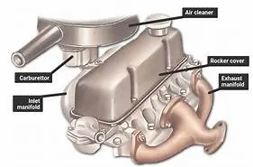
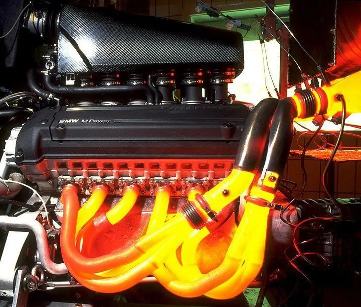
Exhaust Port manifold of BMW inline-6 Engine

The outcome of CHT Analysis:

• Temperature distribution analysis.
• Hear flux rate analysis- calculation of wall heat flux rates or heat transfer coefficients.
• Visualization of heat transfer features for improved understanding of system flow phenomena.
• Identification of localized 'hot spots or heat sinks in checking against specified requirements'.
• Evaluating variation in temperature peaks for different operating conditions/failure modes.
• Assessing insulation or heat shield effectiveness and optimizing of material selections coupling CHT and FE analysis to evaluate thermally induced stresses, expansion or fatigue.

PROCEDURE:

Geometry

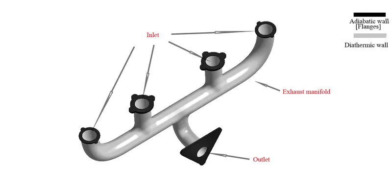
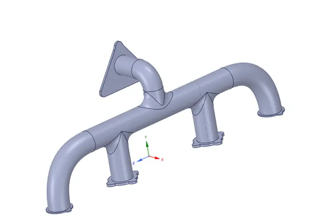
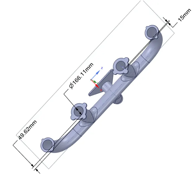
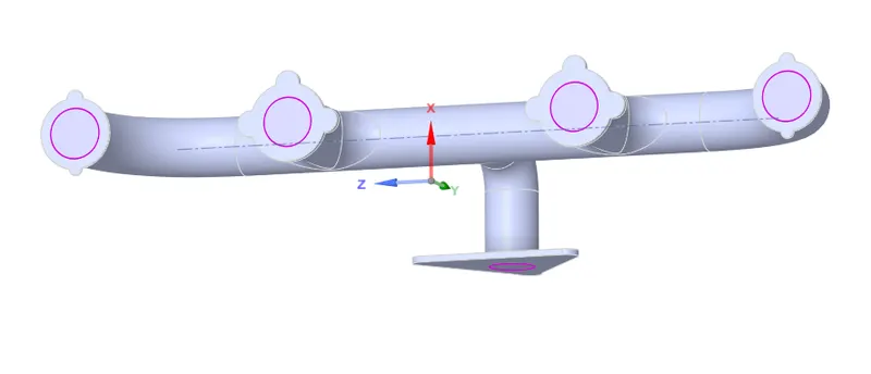
• The modelling and CAD cleanup of Exhaust port is done using ANSYS Spaceclaim.
• In this simulation process, both the solid volume and fluid volume will be required for discretization as wall heat transfer coefficient needs to be evaluated at the shared interface therefore, it is necessary that the solid volume and fluid volume exchange information during the solution process by enabling the share topology option in spaceclaim.

Meshing

• The meshing approach for the given Exhaust port model should be done by taking meshing quality attributes into account such as, Element, skewness, orthogonality and aspect ratio.

Element quality	0-0.15(Bad)	0.16-1.00(Good)
Aspect ratio			Best possible value
Skewness	0-0.25(Excellent)	0.25-0.50(Very good)	0.50-0.80(Good)	0.80-0.94(Acceptable)	0.94-0.97(Bad)	0.97-1.00(Unacceptable)
Orthogonal Quality	0-0.001(Unacceptable)	0.001-0.14(Bad)	0.15-0.20(Acceptable)	0.20-0.69(Good)	0.70-0.95(Very good)	0.95-1.00(Excellent)

• The mesh quality will affect the performance by causing any convergence issues during the solution process and it also helps us to locate areas in the mesh where statistics can be improved.
• First of all, we have to create named selections such as inlet, outlet, and outer-wall-convection.
• we have to create the inflation layer for the fluid volume to capture the viscous effects in the near wall region.
• Calculate the `y` value whether using the skin friction coefficient formula or `y^+` calculator.

Turbulence model:

• From some literature, it is determined that when the flow is fully turbulent , the heat transfer from the boundary layer is maximum.
• For turbulence model associated with energy equation and low Reynolds number should be treated with 2 equation model i.e. K-epsilon or K-omega model. There are more literatures available for choosing either K-epsilon or K-omega models. If we consider the standard K-epsilon model, it is robust turbulence model and used widely despite of limitation of models. But it performs very poorly for complex flows involving pressure gradient, flow separation and strong streamline curvature.
• So another turbulence model in K-epsilon family is Realizable K-epsilon model which can be treated for boundary layer flows with moderate swirls and vortices and locally transitional flows, but the disadvantage is taking more time to converge. The better model compared with K-epsilon is given by standard K-omega model which is most favorable to be used for low Reynolds number flow with wall bounded boundary layer.

So as we have discussed the importance of each turbulence model, we will make some changes with in the simulation cases, all the cases will be simulated with realizable K-epsilon model and standard K-omega model with desirable Y plus value of 50 for both turbulence model. The calculation of total thickness of inflation layer is given below;

1) Calculation of Reynold's number

`Re=((ρ*V*D))/μ=((1.225*5*0.166))/(1.7965E-5)= 56596.1592`

2) Calculation of skin friction coefficient (for internal flow)

`C_f=0.079/(Re^(1/7) )=0.079/(56596.1592)^((1/7) ) =0.01654`

3) Calculatioon of Shear stress near wall

`τ_(wall)=(C_f*ρ*U^2)/2=(0.01654*1.225*(5)^2)/2=0.2532 N/m^2`

4) Calculation of Frictional velocity

`U_(Fric)= √(τ_(wall)/ρ )= √(((0.2532))/((1.225) ))=0.4546`

5) Calculation of first layer thickness

`ΔS=(Y^+*μ)/(U_(Fric)*ρ) =((50*1.78e^(-5) ))/((0.4546*1.225))=0.0016 m`

6) Total thickness of inflation for 5 layers.

Total thickness = `1.6*((1.2)^5) = 3.98 mm`

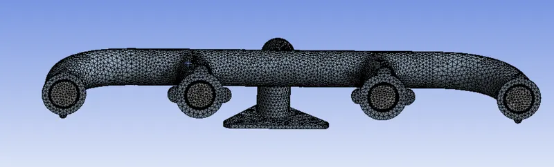
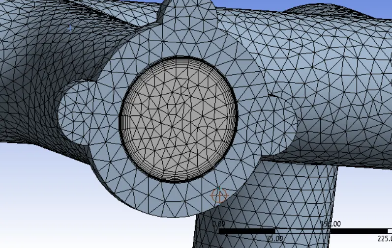
• Element size for solid body: 20mm
• Element size for fluid body: 15mm
• First layer thickness for inflation layer: 1.6mm
• Nodes: 101778
• No. of elements : 339784

Element Quality:

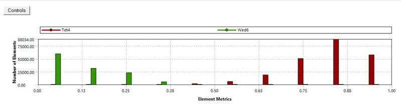
Skewness:

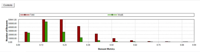
Here, we can see that most of the elements have the skewness close to zero, therefore the mesh is good.

Orthogonality:

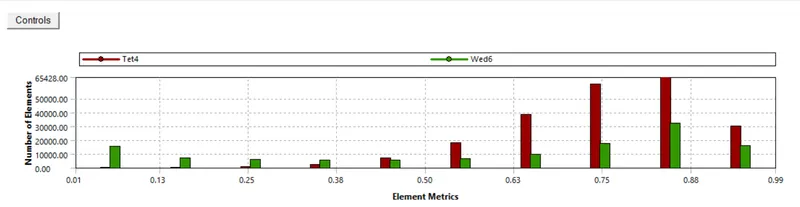
Here also, the orthogonality is close to 1 for maximum elements. so, we can confirm that the mesh is refined.

Calculation of Heat Transfer Coefficient (HTC):-

The calculation of heat transfer coefficient is varying from types of flow to how heat transfer takes place. Calculation of heat transfer coefficient is important in the convection flow because it will provide the value due to which the amount of heat is transferred to the atmosphere due to air motion. calculation of heat transfer coefficient depends upon thermal properties of medium, hydrodynamic characteristic of the flow field and hydrodynamic and thermal boundary conditions. For each mode of heat transfer, there is a provision of dimensionless number which can be used to calculate the heat transfer coefficients. Similarly, there are two methods used by the FLUENT and most other CFD softwares to calculate the heat transfer coefficients , they are ;

• Nearest cell centroid method.
• By input the value of `T_(ref)`

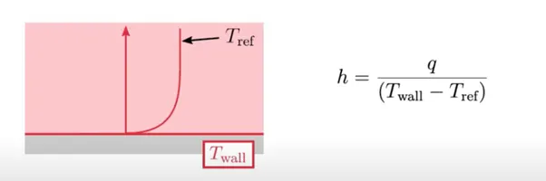
For convective heat transfer calculations if we consider newton's law of cooling , `T_1` is `T_(wall)` and `T_2` is `T_(ref)`. As there is flow field is divided into internal and external flows. In case of external flows, the wall temperature is given by user input as the flow field temperature, but it is necessary to determine the reference temperature. For external flow we can consider the far stream flow temperature as reference temperature as shown in figure:

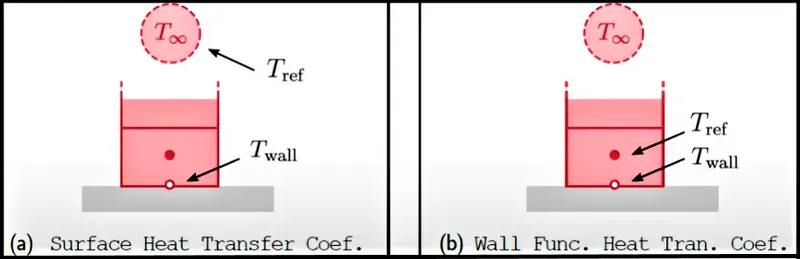
But in case of internal flows, the things get complicated and reference temperature is depending upon the mass-flow average temperature which is given as;

`T_(ref)=1/(m ̇ ) int(ρ U T dA)`

For cell centroid method, the calculation of reference temperature is calculated using Y plus method. In which temperature is considered as function of Y plus value. To calculate the `T^+` value, the equation is given as:

`T^+=(((T_(Wall)-T_(cell) ) ρ C_p C_μ^(1/4) k^0.5 ))/(q )`

We know that, the relation between heat transfer coefficient and cell temperature as the reference temperature which is given as;

`h=q/(T_(Wall)-T_(ref) )`

`∴h=((ρ C_p C_μ^(1/4) k^0.5 ))/T^+`

But we can see that the `T_(ref)` depends on the mesh here,

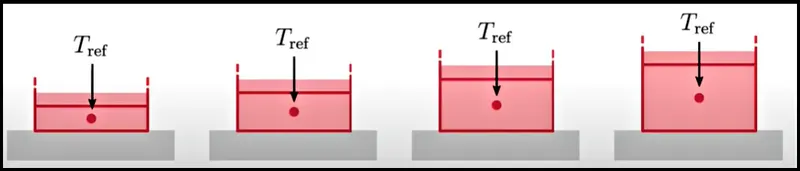
As we said earlier about `T^+` as the function of Y plus value, it is important to determine and calculate the Y plus value for flow domain. The turbulence model also determine what will be the Y plus value for simulation. Using the `K-epsilon` model for the simulation because of two equation model to determine eddy viscosity, the amount of Y plus should be more than 11.25. Considering this mode of turbulence is also good for low Reynold's number flow through pipes. But use of Y plus value to determine the reference temperature `(T_(ref))` to calculate the heat transfer coefficient is more difficult as it will increase the cell count number in simulation. In most of CFD codes like CFX and FLUENT if user knows what is the reference temperature near wall then he can directly provide it in the software. In CFX, it is done using bulk temperature specification and in the FLUENT, it is provided as reference value.

Calculation of HTC ( Analytical soultion):-

We have seen that how CFD code try to calculate the heat transfer coefficient value in the software but it is important to know whether this value which has been calculated from numerical simulation is correct or not. That's why we have to validate the results with the analytical solution. wkt, when Reynold's number is less than 2300 we consider it as laminar flow in the tubes. The Reynolds number formula is given as;

`Re=(ρ V D)/μ`

Where,

ρ is density of fluid

V is fluid velocity

µ is dynamic viscosity of fluid and

D is diameter of tube which can be replaced by L if Reynolds number calculated for the flat plate.

• Here, we are considering that the flow is incompressible with constant properties and fully developed region of a straight circular pipe. It is important to consider the velocity profile as complete in the tube because of characteristic length 'l' which can be further determined by L/D ratio.
• The flow in smooth pipe is fully turbulent for Reynold's number greater than 10000. Most of the time turbulent flow are utilized in the pipe flow because of higher heat transfer coefficients. Most of the correlations of friction and heat transfer are in turbulent flows are based on the experimentation approach because theoretically turbulent flows are difficult to relate.

For Smooth tube:-

The heat transfer coefficient can be calculated by assuming friction factor or directly assuming tube is smooth. For smooth tube, the Darcy friction factor (f) in turbulent flows can be calculated by Petukhov equation which is given as;

for `10^4`<Re<`10^6`

By using the above equaton to determine the friction factor for turbulent flow, the Nusselt number in turbulent flow is given by Chilton-Colburn equation which is given as;

`Nu=0.125*f*Re*(Pr)^(1/3)`

For fully developed turbulent flow in smooth tubes, a simple relation for the Nusselt number is obtained by providing simple substitution of power law for friction factor which is given as;

`f=0.184Re^(-0.2)`

Dittus-Boelter equation:

The Dittus-Boelter equation (for turbulent flow) is an Explicit function for calculating the Nusselt number. It is easy to solve but is less accurate when there is a large temperature difference across the fluid. It is tailored to smooth tubes, so use for rough tubes (most commercial applications) is cautioned.

substitute the friction factor in the nusselt number equation, we get the governed equation of Dittus-Boelter which is given by;

`Nu=0.023 Re^0.8 (Pr)^n`

where:

D is the inside diameter of the circular duct

is the Prandtl number

for the fluid being heated, and for the fluid being cooled.

The Dittus-Boelter equation is valid for

Example:The Dittus-Boelter equation is a good approximation where temperature differences between bulk fluid and heat transfer surface are minimal, avoiding equation complexity and iterative solving. Taking water with a bulk fluid average temperature of 20 °C, viscosity 10.07×10⁻⁴ Pa·s and a heat transfer surface temperature of 40 °C (viscosity 6.96×10⁻⁴, a viscosity correction factor for can be obtained as 1.45. This increases to 3.57 with a heat transfer surface temperature of 100 °C (viscosity 2.82×10⁻⁴ Pa·s), making a significant difference to the Nusselt number and the heat transfer coefficient.

From the Nusselt number, we can calculate the heat transfer coefficient as;

`Nu=h/(k/l)`

Where,

h is heat transfer coefficient (W/m^2k)

k is the thermal conductivity of fluid (W/mk)

and l is characteristic length (m) or D is the diameter of the flow pipe for internal flows (m).

The given data for air as a fluid, the properties of air given as;

• Density of Air = 1.225 Kg/m³
• Dynamic Viscosity = 1.7965E-5 Kg/m.s
• Specific heat = 1.006E+3 J/kgK
• Thermal Conductivity = 0.0252 W/mK
• Prandtl number = 0.7165
• Diameter of Pipe = 0.166 m
• Velocity of Air = 5 m/s

A) Calculation of Reynolds Number:

`Re=((ρ*V*D))/μ=((1.225*5*0.166))/(1.7965E-5)= 56596.1592`

As, we can see that the calculated value for Reynold's number is more than 10000. Hence, the flow is turbulent in nature.

B) Calculation of Nusselt Number:

`Nu=0.023 Re^0.8 (Pr)^n`

`Nu=0.023*(56596.1592)^0.8*(0.7165)^0.3`

`Nu = 131.98`

C) Calculation of Heat Transfer Coefficient:

`Nu=h/(k/l)`

`h=Nu*k/l=131.98*(0.0252/0.166)=20.03 W/m^2 K`

The above calculation is done in respect without consideration of friction factor in this simulation. The calculation which is done is not much accurate, it is evident that considering friction factor will improve the solution which will also increase the heat transfer coefficient. The calculation of heat transfer coefficient with Dittus-Boelter equation provide almost 25% of error which need to be minimized by second Petukhov equation which is given as;

Considering Rough surface:-

Gneilinski's correlation:

Gnielinski's correlation for turbulent flow in tubes:

Where f is the Darcy friction factor that can either be obtained from the Moody chart or for smooth tubes from correlation developed by Petukhov:

The Gnielinski Correlation is valid for:

For the calculation of heat transfer coefficient for above equation it is important to know about roughness of the tube. The roughness can be calculated by using Colebrook equation which depends on Reynold's number and relative roughness `epsilon/D`.

`1/(√(f ))= -2.0 log⁡(((ε/D))/3.7+2.51/(Re* √f))`

If we can associate the value with respect to friction factor equation, the f value will be 0.0312 and substituting the f value in Gnielinski's equation, we can get the Nusselt number as 192.63 and the resultant heat transfer coefficient is around 28.55 `W/(m^2k)`

Hence, from the calculation we can notice that providing friction factor in the calculation of heat transfer coefficient will greatly affect the value at higher side which means more heat transfer through the pipe to the atmosphere. In real life manufacturing, we consider the roughness as no surface which is 100% smooth. Besides, the smooth tube the calculation of HTC using Gneilinski's equation gives only 10% error than the Dittus-Boelter equation.

FLUENT set-up

• Once the mesh is imported, check for mesh to confirm.
• Go on with pressure based solver type as we are dealing with incompressible fluid with mach number less than 0.3 here. And the simulation time is study.
• Velocity formulation - Absolute
• Run the simulation with the default fluid: AIR and solid materials: ALUMINIUM of FLUENT.

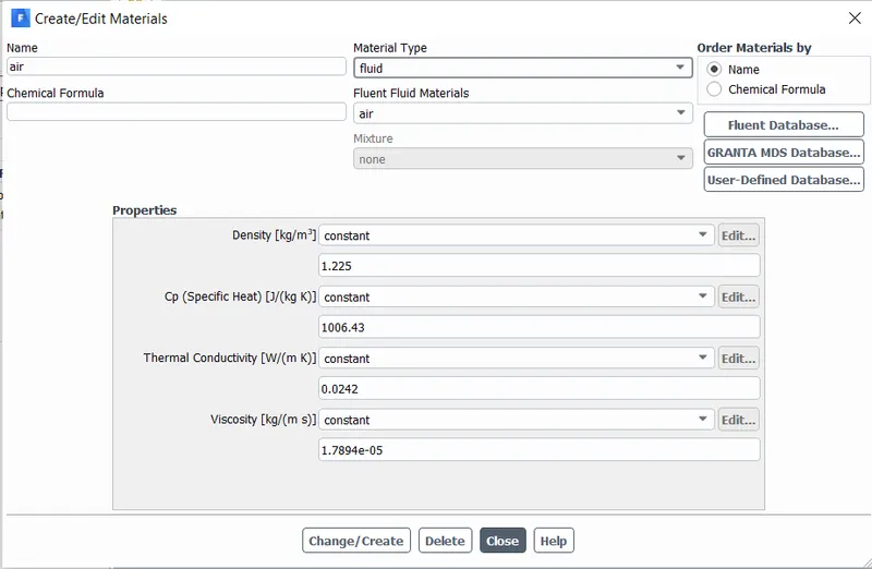
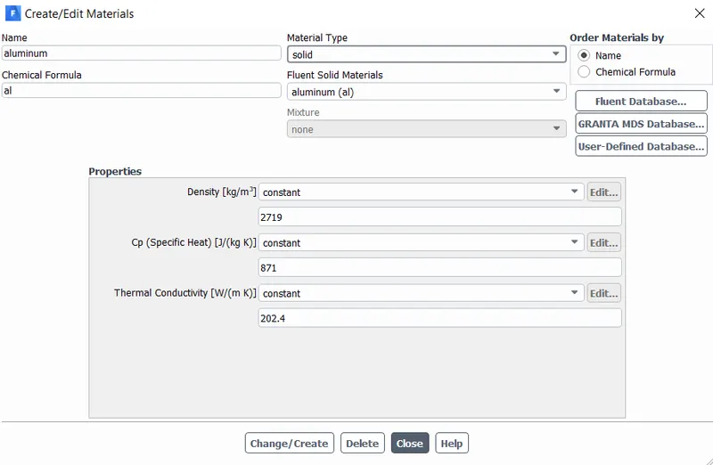
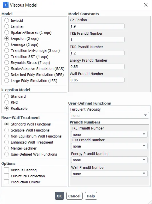
• As discussed earlier, we will go with Realizable K-epsilon viscous model and with the energy equation is activated for energy equations.

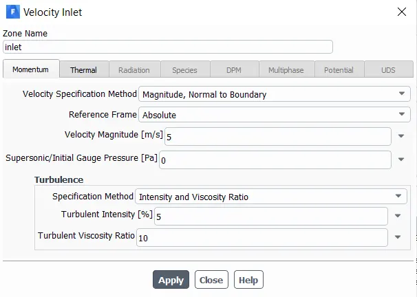
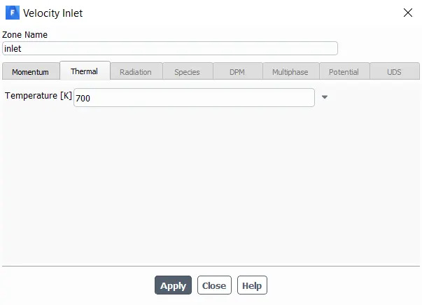
• Set-up the boundary conditions as the inlet boundary condition is velocity inlet with 5m/s and 700K as inlet temperature in exhaust manifold which is shown below;

• outlet - Gauge pressure with 300K temperature
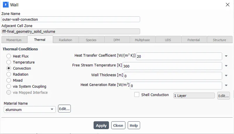
• The outer wall convection has the heat transfer coefficient of 20`W/(m^2K)`

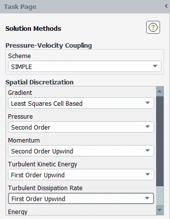
• Moving further for the solution methods, the pressure velocity coupling for the simulation will be considered as SIMPLE for low-Reynold's number flows mostly.

• Initialize the simulation using Hybrid initialization and create the report definitions for Area weighted average of temperature, surface HTC, wall adjacent HTC and Residuals plot.
• Run the simulation for 500 iterations and plot the temperature contour for inlet, outlet and outer wall convection.
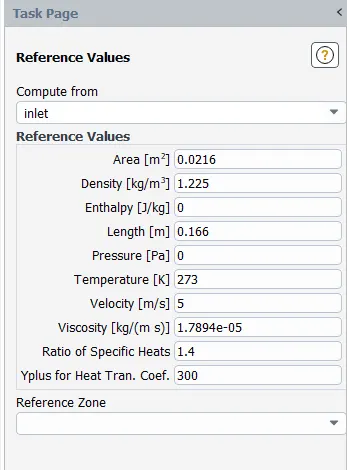
• Set-up the reference value to accurately calculate the heat transfer coefficient and temperature as follows;

RESULTS:

RESIDUAL PLOT

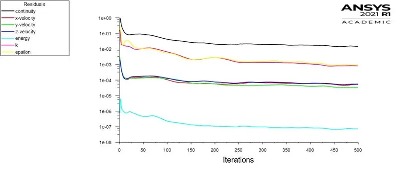
Here, we can see from the residual plot that the results are converging at around 450 to 500 iterations.

AREA WEIGHTED AVERAGE OF TEMPERATURE

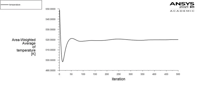
From the above plot it is quite confident that the temperature stabilize at around 400 iterations and the computed area weighted average temperature is 520 degree celsius.

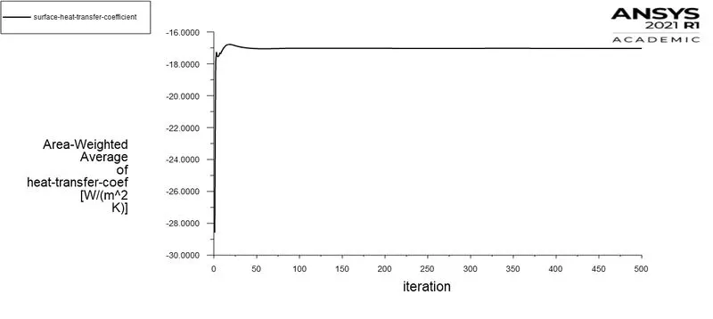
SURFACE HEAT TRANSFER COEFFICIENT

TEMPERATURE CONTOUR ON CONVECTION WALL

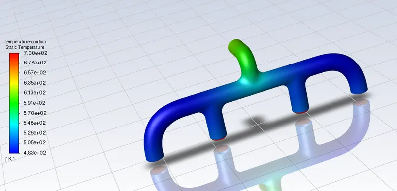
From the above image we can see that, temperature has been stabilized at around 350 iterations and kept constant for almost 150 iterations. We can see temperature distribution very clearly and it is seeming that temperature is higher at where outlet bend has started.

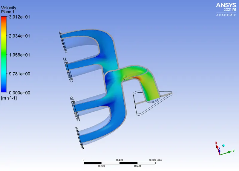
VELOCITY CONTOUR

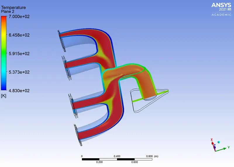
TEMPERATURE CONTOUR

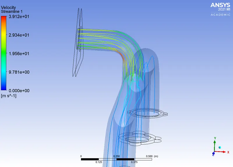
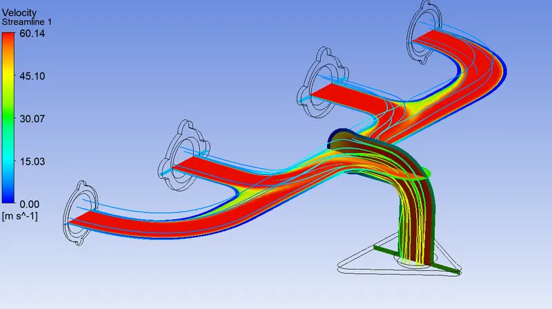
STREAMLINE VELOCITY

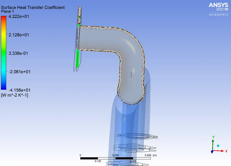
SURFACE HEAT TRANSFER COEFFICIENT

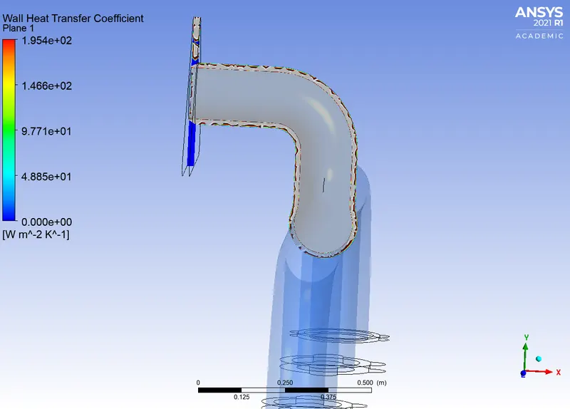
WALL ADJACENT HEAT TRANSFER COEFFICIENT

Case 2:- Inlet velocity of 7.5m/s with inflation- Realizable K-epsilon model.

Analytical calculation of HTC:

A) Calculation of Reynolds Number

`Re=((ρ*V*D))/μ=((1.225*7.5*0.17))/(1.7965E-5)= 86939.88`

As we can see the calculated value for Reynolds number is more than 10000 hence the flow is turbulent in nature.

B) Calculation of Nusselt Number

`Nu=0.023 Re^0.8 (Pr)^n`

`Nu=0.023*(86939.88)^0.8*(0.7165)^0.3`

`Nu=186.066`

C) Calculation of Heat Transfer Coefficienth=Nu⋅kl=186.066⋅(0.02520.17)=27.58Wm2K">

`Nu=h/(k/l)`

`h=Nu*k/l=186.066*(0.0252/0.17)=27.58 W/m^2 K`

Inflation Layer thickness calculation:

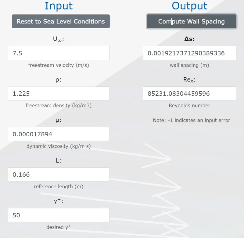
The first layer height of inflation layer for the mesh parameter is 1.92mm and the total thickness is 4.77mm. The mesh after providing inflation is shown below:

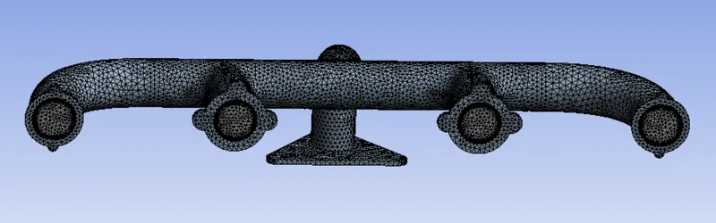
• Nodes: 164093
• Elements: 483095

RESULTS:

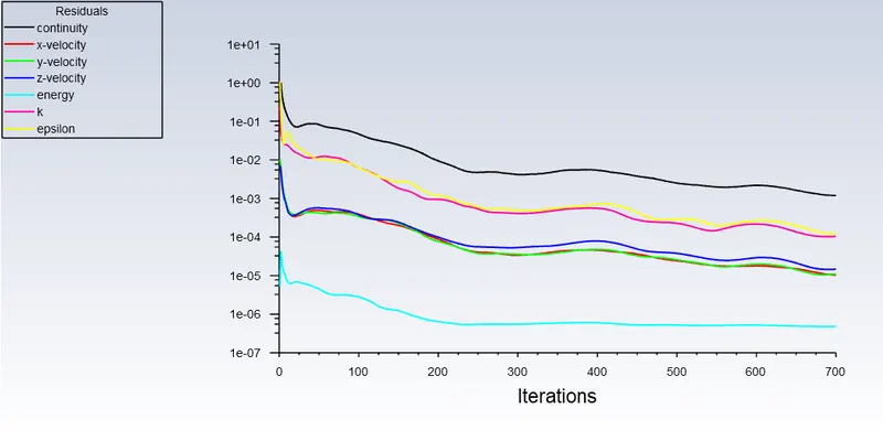
RESIDUAL PLOT

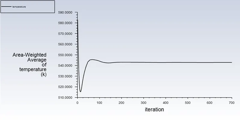
TEMPERATURE PLOT

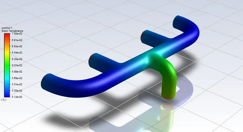
TEMPERATURE CONTOUR ON CONVECTION WALL

TEMPERATURE CONTOUR ON CUT PLANE

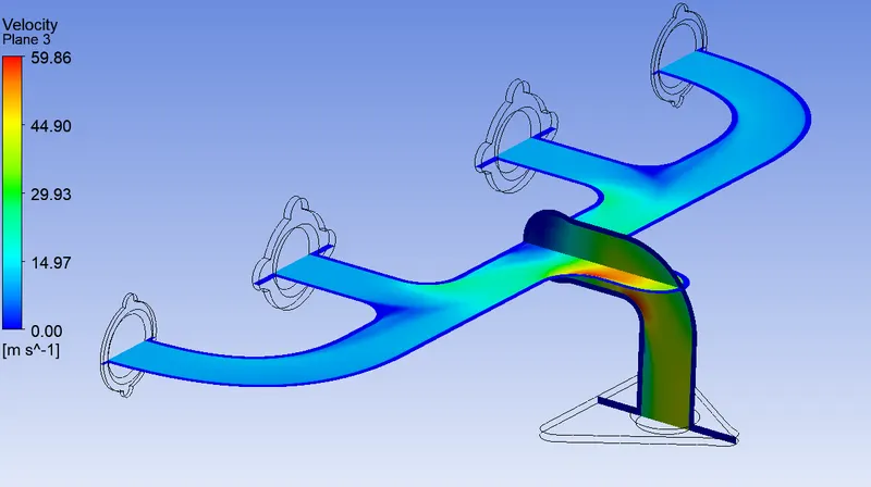
VELOCITY CONTOUR ON CUT PLANE

HEAT TRANSFER COEFFICIENT

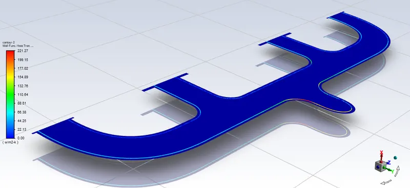
The heat transfer coefficient from CFD simulation is around 28.25 W/m²K. The results are closer to the analytical solution and we can see in above image that as velocity is increased the heat transfer coefficient in the area has also increased because of turbulence.

RESULT TABLE: -

Parameters	Calculated HTC	Simulated HTC	% Error
Case 1	20.03	17.03	14.97
Case 2	27.58	28.25	2.42

CONCLUSION

• From the simulation of exhaust manifold it was evident that the calculated value of heat transfer coefficient are in range of less than 15% error with CFD results. But the simulation has been carried out without considering any friction factor which would have provided better results for cfd simulation.
• The simulation was carried with Realizable K-epsilon model and with different velocities. From the results of residual plot we can say that Relizable K-epsilon model converge faster as compared to Standard K-omega model.
• In all the cases we found that heat transfer coefficient increasing where value of velocity is greater which shows that increasing in turbulence cause the brownian motion to setup and cause fluid particle near to wall accelerate. Providing inflation layer is one of the best mesh input could be utilize for such simulation as we had seen in the baseline simulation it was very difficult to predict the heat transfer coefficient near the wall but after providing inflation we can get better visualization near the wall boundaries.
• For the note on accuracy of prediction of heat transfer coefficient is greatly depend on the velocity of flow means reynolds number and nusselt number. If one calculates the analytical value of heat transfer coefficient and provide similar to simulation then after simulation we can see it matches with calculated value.

REFERENCES:

1) [CFD] Heat Transfer Coefficient (htc) in ANSYS Fluent, OpenFOAM and CFX - YouTube

2) https://www.youtube.com/watch?v=SVYXNICeNWA

3) HEAT TRANSFER COEFFICIENT (thermopedia.com)

4) Yunus A Cengel "Heat Transfer A Practicle Approach"