Week 5.1 - Mid term project - Solving the steady and unsteady 2D heat conduction problem
AIM:
To solve the 2D heat conduction equation(steady and transient)by using the point iterative techniques such as Jacobi, Gauss-seidal and Successive over Relaxation(SOR) methods.
GIVEN:
Top Boundary(TT) = 600 K
Bottom Boundary(TB) = 900 K
Left Boundary(TL) = 400 K
Right Boundary(TR)= 800 K
Error criteria=1e-4
SOLVING THE STEADY STATE EQUATION OF 2D HEAT CONDUCTION:
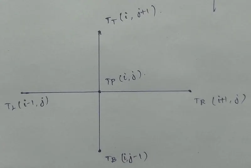
Steady state equation:`(del^2T)/(delx^2)+(del^2T)/(dely^2)=0`
By using central differencing,
`(T_(i+1,j)^n-2T_(i,j)^n+T_(i-1,j)^n)/ (Deltax^2) + (T_(i,j+1)^n-2T_(i,j)^n+T_(i,j-1)^n)/ (Deltay^2) = 0`
On simplification;put
T_(i+1,j)^n= TL,
T_(i-1,j)^n= TR,
T_(i,j+1)^n= TT,
T_(i,j-1)^n= TB,
T_(i,j)^n= TP
we get,
`T_P(2(Deltax^2+Deltay^2)/(Deltax^2.Deltay^2))=((T_L+T_R)/(Deltax^2)+(T_T+T_B)/(Deltay^2))`
`Tp=(1/k)((T_L+T_R)/(Deltax^2)+(T_T+T_B)/(Deltay^2))`
where k= `(2(Deltax^2+Deltay^2)/(Deltax^2.Deltay^2))`
CODE FOR STEADY STATE PROBLEM SOLUTION(IMPLICIT METHOD):
% Solving Steady state 2D heat conduction problem using jacobi, Gauss-Seidal,SOR
% methods
clear all
close all
clc

%2D heat conduction
%Length of domain
L=1;
%number of nodes
nx=10;
ny=nx;

% Grid spacing
x=linspace(0,L,nx);
y=linspace(0,L,ny);
dx=x(2)-x(1);
dy=y(2)-y(1);

%Applying Boundary conditions
T=ones(nx,ny);
T(:,1)=400;
T(:,10)=800;
T(1,:)=600;
T(10,:)=900;
T(1,1)=(600+400)/2;
T(1,10)=(600+800)/2;
T(10,1)=(900+400)/2;
T(10,10)=(800+900)/2;

% copy of temperature value
Told=T;
% value of k
k=2*((dx^2+dy^2)/((dx^2)*(dy^2)));

iterative_solver=3;
error=9e9;
tolerance=1e-4;

% Using jacobi method
if iterative_solver==1
    tic % to calculate simulation time
    jacobi_iteration=1;
    % convergence loop
    while(error>tolerance)
    % spacial loop
        for i=2:nx-1
        for j=2:ny-1

            H=((Told(i-1,j)+Told(i+1,j))/(dx^2));
            V=((Told(i,j-1)+Told(i,j+1))/(dy^2));
            T(i,j)=(H+V)/k;
        end
        end
     % error finding
     error=max(max(abs(Told-T)));
     % Updating the Told value
     Told=T;
     jacobi_iteration=jacobi_iteration+1;
    end

iteration_time=toc;
figure(1)
contourf(x,y,T);
[a,b]=contourf(x,y,T);
colormap(jet);
clabel(a,b);
colorbar
xlabel('X axis')
ylabel('Y axis')
set(gca,'YDIR','reverse');
title_text=sprintf('Number of iterations=%d iteration time=%d',jacobi_iteration,iteration_time);
title(title_text)
saveas(gca,'Jacobi Iteration Steady state.jpg')
end

% Using Gauss-Seidal method
if iterative_solver==2
    tic
    GS_iteration=1;
    while(error>tolerance)
        for i=2:nx-1
            for j=2:ny-1

            H=((T(i-1,j)+T(i+1,j))/(dx^2));
            V=((T(i,j-1)+T(i,j+1))/(dy^2));
            T(i,j)=(H+V)/k;
            end
        end
        error=max(max(abs(Told-T)));
        Told=T; % updating the Told value
        GS_iteration= GS_iteration+1;
    end
    iteration_time=toc;
    figure(2)
    contourf(x,y,T)
    [a,b]=contourf(x,y,T);
    colormap(jet);
    clabel(a,b);
    xlabel('X axis')
    ylabel('Y axis')
    set(gca,'YDIR','reverse');
    colorbar
    title_text=sprintf('Number of iterations=%d iteration time=%d',GS_iteration,iteration_time);
    title(title_text);
    saveas(gca,'Gauss seidal steady state.jpg')
end

%Relaxation factor
omega=1.1;
% Using Successive-over Relaxation(SOR)method
if iterative_solver==3
    tic
    SOR_iteration=1;
    while(error>tolerance)
        for i=2:nx-1
            for j=2:ny-1

                H=((T(i-1,j)+T(i+1,j))/(dx^2));
                V=((T(i,j-1)+T(i,j+1))/(dy^2));
                T(i,j)=(1-omega)*Told(i,j)+(omega*((H+V)/k));
            end
        end
            error=max(max(abs(Told-T)));
            Told=T;
            SOR_iteration=SOR_iteration+1;
    end
    iteration_time=toc;
    figure(3)
    contourf(x,y,T)
    [a,b]=contourf(x,y,T);
    colormap(jet);
    clabel(a,b);
    xlabel('X axis')
    ylabel('Y axis')
    set(gca,'YDIR','reverse');
    colorbar
    title_text=sprintf('Number of iterations=%d iteration time=%d',SOR_iteration,iteration_time);
    title(title_text);
    saveas(gca,'SOR steady state.jpg')
end
OUTPUT:
1. JACOBI METHOD
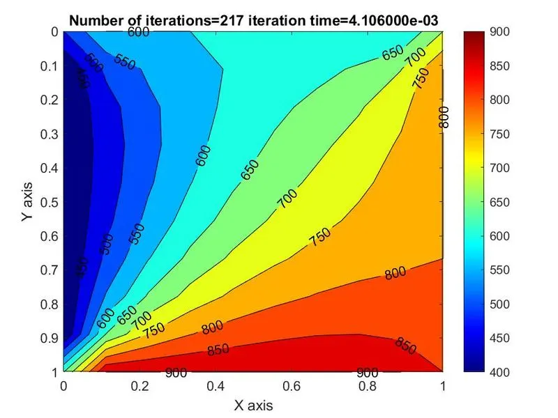
The time required for convergence is 4.106e-3 sec and Number of iterations took to converage is 217 which is the highest number of iterations in steady state solution.
2. GAUSS SEIDAL METHOD.
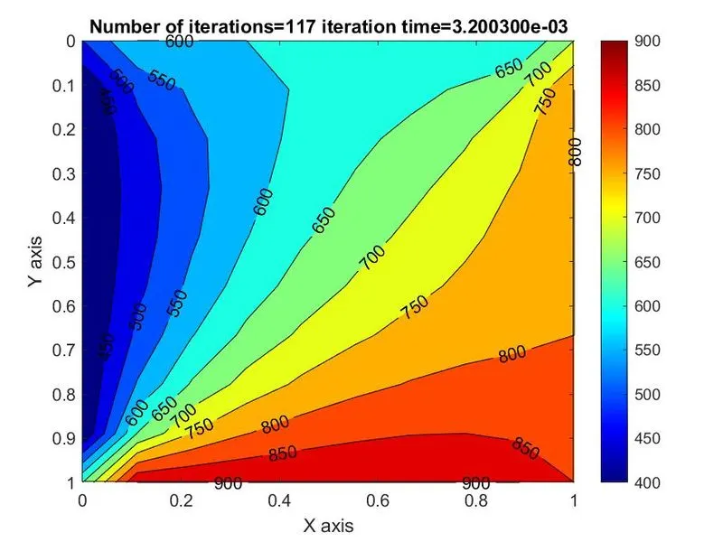
The time required for convergence is 3.20e-3 sec and number of iterations carried out are 117 which much less than the jacobi method for convergence to take place.
3. SOR METHOD
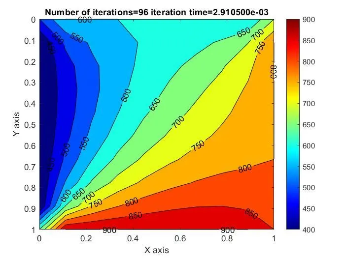
The time required for convergence 2.91e-3 sec and iterations carried out are 96 which is the lowest number of iterations in steady state solution . Therefore, the SOR method is the fastest method to reach convergence among the iterative solvers. Also, in the SOR method , by increasing the relaxation factor omega to 1.2, 1.3,..1.5 ,it is seen that the number of iterations reduces from 96 to 30 iterations.For omega=1.6, the number of iterations increases to 38, that is called over relaxation.
SOLVING THE TRANSIENT STATE EQUATION OF 2D HEAT CONDUCTION:
Unsteady or Transient state Equation: `(delT)/(delt)=alpha((del^2T)/(delx^2)+(del^2T)/(del y^2))`
By forward differencing the temporal terms LHS: we get,
`(delT)/(delt)=(T^(n+1)i,j-T^ni,j)/(Delta t)`
Using central differencing for the spacial terms,
`(del^2T)/(delx^2)=(T_(i-1,j)-2T_(i,j)+T_(i+1,j))/(Deltax^2)`
`(del^2T)/(dely^2)=(T_(i,j-1)-2T_(i,j)+T_(i,j+1))/(Deltay^2)`
On simplification;put
T_(i+1,j)^n= TL,
T_(i-1,j)^n= TR,
T_(i,j+1)^n= TT,
T_(i,j-1)^n= TB,
T_(i,j)^n= TP
we get,
`T_P^(n+1) = T_P^n + alpha*Deltat[(T_R^n - 2T_P^n + T_L^n)/(Deltax^2) + (T_T^n - 2T_P^n + T_B^n)/(Deltay^2)]`
`T_P^(n+1) = T_P^n(1-2k_1-2k_2) + k_1T_L^n+ k_1T_R^n + k_2T_B^n + k_2T_T^n`
where, `k_1 =( alpha*Deltat)/(Deltax^2)`and
`k_2 = ( alpha*Deltat)/(Deltay^2)`
The Equation for Explicit form;
`Tp^(n+1)=Tp^n*(1-2k1-2k2)+k1(TL+TR)^n+k2(T T+TB)^n`
The Equation for implicit form;
`Tp^(n+1)=(Tp^n+k1(TL+TR)^(n+1)+k2(T T+TB)^(n+1))/(1+2k1+2k2)`
CODE FOR TRANSIENT STATE PROBLEM SOLUTION:
1. Explicit Method:
% Solving Unsteady state(Transient) 2D heat conduction problem
% Explicit method for Transient solution
clear all
close all
clc

%Length of domain
L=1;
%number of nodes
nx=10;
ny=nx;

%grid spacing
x=linspace(0,L,nx);
y=linspace(0,L,ny);
dx=x(2)-x(1);
dy=y(2)-y(1);

%defining the temperature terms
alpha=1.4;
nt=1400;
dt=0.001;

%Applying Boundary conditions
T=ones(nx,ny);
T(:,1)=400;
T(:,10)=800;
T(1,:)=600;
T(10,:)=900;
%defining edges of the T
T(1,1)=(600+400)/2;
T(1,10)=(600+800)/2;
T(10,1)=(900+400)/2;
T(10,10)=(800+900)/2;

%CFL value
k1=alpha*(dt/(dx^2));
k2=alpha*(dt/(dy^2));

error=9e9;
tolerance=1e-4;
% copy of temperature value
Told=T;

%Explicit calculation
Explicit_iteration=1;
%Time loop
tic
for t=1:nt
    %spacial loop
    for i=2:nx-1
        for j=2:ny-1

            term_1=(1-2*k1-2*k2);
            term_2=k1;
            term_3=k2;
            H=(Told(i+1,j)+Told(i-1,j));
            V=(Told(i,j+1)+Told(i,j-1));
            T(i,j)=(Told(i,j)*term_1)+(term_2*H)+(term_3*V);
        end
    end
    Told=T;
    Explicit_iteration=Explicit_iteration+1;
end
iteration_time=toc;
figure(1)
contourf(x,y,T);
[a,b]=contourf(x,y,T);
colormap(jet);
clabel(a,b);
colorbar
xlabel('X axis')
ylabel('Y axis')
set(gca,'YDIR','reverse');
title_text=sprintf('Number of iterations=%d iteration time=%d',Explicit_iteration,iteration_time);
title(title_text)
saveas(gca,'Explicit iteration Unsteady state.jpg')
OUTPUT:
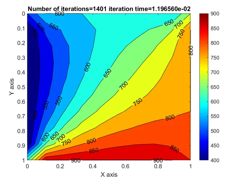
The iterations required to converge the simulation is 1401 and time is 1.1965e-2 sec. If we decrease or increase other than 0.0001, the solution will become unstable. Also, the explicit scheme takes less time than any other implicit scheme methods.
2. Implicit Method:
% solution for Transient state problem using implicit method
clear all
close all
clc

%Length of domain
L=1;
%number of nodes
nx=10;
ny=nx;

%grid spacing
x=linspace(0,L,nx);
y=linspace(0,L,ny);
dx=x(2)-x(1);
dy=y(2)-y(1);

%defining the temperature terms
alpha=1.4;
nt=1400;
dt=0.001;

%Applying Boundary conditions
T=ones(nx,ny);
T(:,1)=400;
T(:,10)=800;
T(1,:)=600;
T(10,:)=900;
%defining edges of the T
T(1,1)=(600+400)/2;
T(1,10)=(600+800)/2;
T(10,1)=(900+400)/2;
T(10,10)=(800+900)/2;

%CFL value
k1=alpha*(dt/(dx^2));
k2=alpha*(dt/(dy^2));
CFL=k1+k2;

error=9e9;
tolerance=1e-4;

% copy of temperature value
Told=T;
Tprev_dt=T;

iterative_solver=1;

%jacobi method
tic
if iterative_solver==1
    jacobi_iteration=1;
    %time loop
    for t=1:nt
        error=9e9;
        %convergence loop
        while(error>tolerance)
            %spacial loop
            for i=2:nx-1
                for j=2:ny-1

                    term_1=(1+(2*k1)+(2*k2))^-1;
                    term_2=k1*term_1;
                    term_3=k2*term_1;
                    H=(Told(i+1,j)+Told(i-1,j));
                    V=(Told(i,j+1)+Told(i,j-1));
                    T(i,j)=(Tprev_dt(i,j)*term_1)+(term_2*H)+(term_3*V);
                end
            end
            error=max(max(abs(Told-T)));
            Told=T;
            jacobi_iteration=jacobi_iteration+1;
        end
        Tprev_dt=T;
    end
iteration_time=toc;
figure(1)
contourf(x,y,T);
[a,b]=contourf(x,y,T);
colormap(jet);
clabel(a,b);
colorbar
xlabel('X axis')
ylabel('Y axis')
set(gca,'YDIR','reverse');
title_text=sprintf('Number of iterations=%d iteration time=%d',jacobi_iteration,iteration_time);
title(title_text)
saveas(gca,'Jacobi Iteration Unsteady state.jpg')
end

%Gauss_Seidal method
tic
if iterative_solver==2
    GS_iteration=1;
    %time loop
    for t=1:nt
        error=9e9;
        %convergence loop
        while(error>tolerance)
            %spacial loop
            for i=2:nx-1
                for j=2:ny-1

                    term_1=(1+2*k1+2*k2)^-1;
                    term_2=k1*term_1;
                    term_3=k2*term_1;
                    H=(Told(i+1,j)+T(i-1,j));
                    V=(Told(i,j+1)+T(i,j-1));
                    T(i,j)=(Tprev_dt(i,j)*term_1)+(term_2*H)+(term_3*V);
                end
            end
            error=max(max(abs(Told-T)));
            Told=T;
            GS_iteration=GS_iteration+1;
        end
        Tprev_dt=T;
    end
iteration_time=toc;
figure(2)
contourf(x,y,T);
[a,b]=contourf(x,y,T);
colormap(jet);
clabel(a,b);
colorbar
xlabel('X axis')
ylabel('Y axis')
set(gca,'YDIR','reverse');
title_text=sprintf('Number of iterations=%d iteration time=%d',GS_iteration,iteration_time);
title(title_text)
saveas(gca,'GS Iteration Unsteady state.jpg')
end

%Relaxation factor
omega=1.2;
%Successive-over Relaxation(SOR)method
tic
if iterative_solver==3
    SOR_iteration=1;
    %time loop
    for t=1:nt
        error=9e9;
        %convergence loop
        while(error>tolerance)
            %spacial loop
            for i=2:nx-1
                for j=2:ny-1

                    term_1=(1+2*k1+2*k2)^-1;
                    term_2=k1*term_1;
                    term_3=k2*term_1;
                    H=(Told(i+1,j)+T(i-1,j));
                    V=(Told(i,j+1)+T(i,j-1));
                    T(i,j)=((1-omega)*Told(i,j))+(omega*((Tprev_dt(i,j)*term_1)+(term_2*H)+(term_3*V)));
                end
            end
            error=max(max(abs(Told-T)));
            Told=T;
            SOR_iteration=SOR_iteration+1;
        end
        Tprev_dt=T;
    end
iteration_time=toc;
figure(3)
contourf(x,y,T);
[a,b]=contourf(x,y,T);
colormap(jet);
clabel(a,b);
colorbar
xlabel('X axis')
ylabel('Y axis')
set(gca,'YDIR','reverse');
title_text=sprintf('Number of iterations=%d iteration time=%d',SOR_iteration,iteration_time);
title(title_text)
saveas(gca,'SOR Iteration Unsteady state.jpg')
end
OUTPUT:
1. Jacobi method
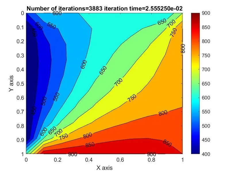
The time required for convergence is 2.555e-2 sec and Iterations carried out are 3883 which is the highest number of iterations in Transient-state solution.
2. Gauss-Siedal Method
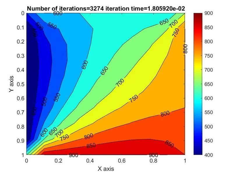
The time required for convergence is 1.8059e-2 sec and number of iterations carried out are 3274 which is pretty much less than iterations of jacobi method solution in Transient-state.
3. SOR Method
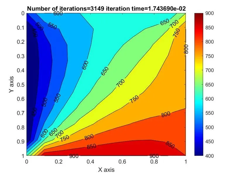
The time required for convergence is 1.74369e-2 sec and number of iterations carried out are 3149 which is the lowest number of iterations in Transient-state solution. Also, it is the fastest method in implicit schemes because the iteration time is faster than other two schemes.
CONCLUSION:
1. The steady-state solution is the fastest schemes to compute the solution because the absence of time derivative term and diffusivity in the equation which leads to faster computation.
2. Explicit scheme forms to be the fastest among the transient state problem. It requires way less number of iterations and computation time to converge compared to Implicit schemes.
3. Relaxation factor (omega) must be maintained within the range of 1.1 to 1.3. More or less than the range it may become over-relaxed or under-relaxed.
4. From obsevation of the reults, all the iterative solvers reach convergence.However, Jacobi method takes most computational time and iterations whereas SOR takes the least time and No. of iterations is less than both the jacobi and GS iterations.
5. From the results, we can conclude the SOR enhances the solution fastest and in least number of iterations.
6. The implicit scheme performs most iterations amongst the steady state and transient state.
7. Implicit scheme gives better results as compared to the explicit scheme in any of the iterative solvers.