Week 3.5 - Deriving 4th order approximation of a 2nd order derivative using Taylor Table method
AIM:
To Derive the following 4th order Approximations of the second-order derivative.
a) Skewed Right-sided difference
b) Skewed Left-sided difference
c) Central difference
Deriving the 4th order approximations of the second-order derivative
1. Skewed Right-sided difference:
The number of nodes required for the 4th order approximation of a second order derivative can be given by the equation
N = P+Q = 2+4=6
where, N is the number of nodes
Q is the order of derivative
P is the order of Approximation.
so, Here we need 6 nodes in order to find the 4th order Approximation of the second-order derivative.
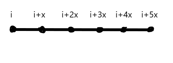
consider the value of `del^2f/(del x^2)` with the 4th order of approximation is given by the equation,
`del^2f/(del x^2)= af(i)+bf(i+1)+cf(i+2)+df(i+3)+ef(i+4)+gf(i+5)`
Now, using the taylor series to find the values of discrete points with respect to point 'i'.
`af(i)=af(i)`
`bf(i+1)=bf(i)+b Delta x f'(i)+b Deltax^2/2 f''(i)+b Deltax^3/6 f'''(i)+b Deltax^4/24 f''''(i)+b Deltax^5/120 f'''''(i)+b Deltax^6/720 f''''''(i)+...`
`cf(i+2)= cf(i)+c(2 Deltax)f'(i)+c(2 Deltax)^2/2.f''(i)+c(2 Delta x)^3/6.f'''(i)+c(2 Delta x)^4/24.f''''(i)+c(2 Delta x)^5/120.f'''''(i)+c(2 Delta x)^6/720.f''''''(i)+...`
`df(i+3)= df(i)+d(3 Deltax)f'(i)+d(3 Deltax)^2/2.f''(i)+d(3 Delta x)^3/6.f'''(i)+d(3 Delta x)^4/24.f''''(i)+d(3 Delta x)^5/120.f'''''(i)+d(3 Delta x)^6/720.f''''''(i)+...`
`ef(i+4)= ef(i)+e(4 Deltax)f'(i)+e(4 Deltax)^2/2.f''(i)+e(4 Delta x)^3/6.f'''(i)+e(4 Delta x)^4/24.f''''(i)+e(4 Delta x)^5/120.f'''''(i)+e(4 Delta x)^6/720.f''''''(i)+...`
`gf(i+5)= gf(i)+g(5 Delta x)f'(i)+g(5 Deltax)^2/2.f''(i)+g(5 Delta x)^3/6.f'''(i)+g(5 Delta x)^4/24.f''''(i)+g(5 Delta x)^5/120.f'''''(i)+g(5 Delta x)^6/720.f''''''(i)+...`
Adding LHS and RHS of the above equations , we get
af(i)+bf(i+1)+cf(i+2)+df(i+3)+ef(i+4)+gf(i+5)= `f(i)[a+b+c+d+e+g]+Delta x f'(i)[b+2c+3d+4e+5g]+Delta x^2f''(i)[b/2+4c/2+9d/2+16e/2+25g/2]+Delta x^3 f'''(i)[b/6+8c/6+27d/6+64e/6+125g/6]+ Delta x^4 f''''(i)[b/24+16c/24+81d/24+256e/24+625g/24]+ Delta x^5 f'''''(i)[b/120+32c/120+243d/120+1024e/120+3125g/120]+ Delta x^6 f''''''(i)[b/720+64c/720+729d/720+4096e/720+15625g/720]`
In the above equations,we only want the co-efficients of `Delta x^2 f''(i)`and we assume coefficient to be one for f''(i) and zero for the rest of all.
Therefore ,the six equations are;
`[a+b+c+d+e+g]=0---(1)`
`[b+2c+3d+4e+5g]=0---(2)`
`[b/2+4c/2+9d/2+16e/2+25g/2]=1---(3)`
`[b/6+8c/6+27d/6+64e/6+125g/6]=0---(4)`
`[b/24+16c/24+81d/24+256e/24+625g/24]=0---(5)`
`[b/120+32c/120+243d/120+1024e/120+3125g/120]=0---(6)`
`[b/720+64c/720+729d/720+4096e/720+15625g/720]=0`
|
Taylor Table |
||||||||
|
Assumed Function |
Taylor Series Expansion |
|||||||
|
`f(i)` |
`Deltax f'(i)` |
`Deltax^2 f''(i)` |
`Deltax^3f'''(i)` |
`Deltax^4 f''''(i)` |
`Deltax^5 f'''''(i)` |
`Deltax^6 f''''''(i)` |
||
|
Stencil |
af(i) |
a |
0 |
0 |
0 |
0 |
0 |
0 |
|
bf(i+1) |
b |
b |
b/2 |
b/6 |
b/24 |
b/120 |
b/720 |
|
|
cf(i+2) |
c |
2c |
4c/2 |
8c/6 |
16c/24 |
32c/120 |
64c/720 |
|
|
df(i+3) |
d |
3d |
9d/2 |
27e/6 |
81d/24 |
243d/120 |
729d/720 |
|
|
ef(i+4) |
e |
4e |
16e/2 |
64e/6 |
256e/24 |
1024e/120 |
4096e/720 |
|
|
gf(i+5) |
g |
5g |
25g/2 |
125g/6 |
625g/24 |
3125e/120 |
15625g/720 |
|
|
Sum of co-efficients `del^2f/(del x^2)` |
0 |
0 |
1 |
0 |
0 |
0 |
? |
|
Writing the coefficients in the form of a matrix , we get
`[[1,1,1,1,1,1],[0,1,2,3,4,5],[0,1/2,4/2,9/2,16/2,25/2],[0,1/6,8/6,27/6,64/6,125/6],[0,1/24,16/24,81/24,256/24,625/24],[0,1/120,32/120,243/120,1024/120,3125/120]]``.[[a],[b],[c],[d],[e],[g]]=[[0],[0],[1],[0],[0],[0]]`
Solving the above matrix form using AX=B in MATLAB to find the values of coefficients
A=[1 1 1 1 1 1;0 1 2 3 4 5;0 1/2 4/2 9/2 16/2 25/2;0 1/6 8/6 27/6 64/6 125/6;0 1/24 16/24 81/24 256/24 625/24;0 1/120 32/120 243/120 1024/120 3125/120];

B=[0;0;1;0;0;0];

x=inv(A)*B;
we get,
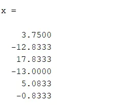
After solving the above matrix , we get the values of coefficients as
a= 3.7500, b= -12.8333, c= 17.8333, d= -13.0000, e= 5.0833, g= -0.8333
Now, dividing both sides of the Hypothesis Eqn.(1) by `(Deltax^2)`; we get,
The Equation using the Taylor table as;
`del^2f/(delx^2)=(af(i)+bf(i+1)+cf(i+2)+df(i+3)+ef(i+4)+gf(i+5))/(Deltax^2)`
Now, from our Taylor table:
`(del^2f)/(delx^2)=(a+b+c+d+e+g)f(i)+(0+b+2c+3d+4e+5g)f'(i)Deltax+(0+b/2+4c/2+9d/2+16e/2+25g/2)f''(i)Delta x^2+(0+b/6+8c/6+27d/6+64e/6+125g/6)f'''(i) Delta x^3+(0+b/24+16c/24+81d/24+256e/24+625g/24)f''''(i)Deltax^4+(0+b/120+32c/120+243d/120+1024e/120+3125g/120)f'''''(i)Delta x^5+(0+b/720+64c/720+729d/72+4096e/720+15625g/720)f''''''(i) Deltax^6`
On dividing the above equation by `(Deltax^2)`, we get;
`(del^2f)/(delx^2)=(b/2+2c+9d/2+8e+25g/2)f''(i)+(b/720+64c/720+729d/720+4096e/720+15625g/720)f'''''(i) Delta x^4`
As, we discussed earlier, the `Delta x^4`denotes the truncation error. Here, we can see that order of the truncation error;`[0(Delta x^4)]`is '4'. Since, we know that the order of approximation is defined by the truncation error term. Therefore, we can say that out skewed right-sided difference scheme is of 4th order accurate.
2. Skewed Left-sided Difference:
The number of nodes required for the 4th order approximation of a second order derivative can be given by the equation
N = P+Q = 2+4=6
where, N is the number of nodes
Q is the order of derivative
P is the order of Approximation.
so, Here we need 6 nodes in order to find the 4th order Approximation of the second-order derivative.
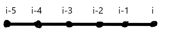
According to the above stencil, The Hypothesis Equation will be,
`del^2f/(del x^2)= af(i)+bf(i-1)+cf(i-2)+df(i-3)+ef(i-4)+gf(i-5)`
Writing Taylor series Expansion for Hypothesis Equation
`af(i)=af(i)`
`bf(i-1)=bf(i)-b Delta x f'(i)+b Deltax^2/2 f''(i)-b Deltax^3/6 f'''(i)+b Deltax^4/24 f''''(i)-b Deltax^5/120 f'''''(i)+b Deltax^6/720 f''''''(i)-...`
`cf(i-2)= cf(i)-c(2 Deltax)f'(i)+c(2 Deltax)^2/2.f''(i)-c(2 Delta x)^3/6.f'''(i)+c(2 Delta x)^4/24.f''''(i)-c(2 Delta x)^5/120.f'''''(i)+c(2 Delta x)^6/720.f''''''(i)-...`
`df(i-3)= df(i)-d(3 Deltax)f'(i)+d(3 Deltax)^2/2.f''(i)-d(3 Delta x)^3/6.f'''(i)+d(3 Delta x)^4/24.f''''(i)-d(3 Delta x)^5/120.f'''''(i)+d(3 Delta x)^6/720.f''''''(i)-...`
`ef(i-4)= ef(i)-e(4 Deltax)f'(i)+e(4 Deltax)^2/2.f''(i)-e(4 Delta x)^3/6.f'''(i)+e(4 Delta x)^4/24.f''''(i)-e(4 Delta x)^5/120.f'''''(i)+e(4 Delta x)^6/720.f''''''(i)-...`
`gf(i-5)= gf(i)-g(5 Delta x)f'(i)+g(5 Deltax)^2/2.f''(i)-g(5 Delta x)^3/6.f'''(i)+g(5 Delta x)^4/24.f''''(i)-g(5 Delta x)^5/120.f'''''(i)+g(5 Delta x)^6/720.f''''''(i)-...`
Now, arranging the above taylor series Expansion in taylor table,we get
Consider Taylor table for left-sided difference.
|
Taylor Table |
||||||||
|
Assumed Function |
Taylor Series Expansion |
|||||||
|
`f(i)` |
`Deltax f'(i)` |
`Deltax^2 f''(i)` |
`Deltax^3f'''(i)` |
`Deltax^4 f''''(i)` |
`Deltax^5 f'''''(i)` |
`Deltax^6 f''''''(i)` |
||
|
Stencil |
af(i) |
a |
0 |
0 |
0 |
0 |
0 |
0 |
|
bf(i-1) |
b |
-b |
b/2 |
-b/6 |
b/24 |
-b/120 |
b/720 |
|
|
cf(i-2) |
c |
-2c |
4c/2 |
-8c/6 |
16c/24 |
-32c/120 |
64c/720 |
|
|
df(i-3) |
d |
-3d |
9d/2 |
-27d/6 |
81d/24 |
-243d/120 |
729d/720 |
|
|
ef(i-4) |
e |
-4e |
16e/2 |
-64e/6 |
256e/24 |
-1024e/120 |
4096e/720 |
|
|
gf(i-5) |
g |
-5g |
25g/2 |
-125g/6 |
625g/24 |
-3125g/120 |
15625g/720 |
|
|
Sum of co-efficients `del^2f/(del x^2)` |
0 |
0 |
1 |
0 |
0 |
0 |
? |
|
Therefore ,the six equations are;
`[a+b+c+d+e+g]=0---(1)`
`[-b-2c-3d-4e-5g]=0---(2)`
`[b/2+4c/2+9d/2+16e/2+25g/2]=1---(3)`
`[-b/6-8c/6-27d/6-64e/6-125g/6]=0---(4)`
`[b/24+16c/24+81d/24+256e/24+625g/24]=0---(5)`
`[-b/120-32c/120-243d/120-1024e/120-3125g/120]=0---(6)`
`[b/720+64c/720+729d/720+4096e/720+15625g/720]=0`
Writing the coefficients in the form of a matrix , we get
`[[1,1,1,1,1,1],[0,-1,-2,-3,-4,-5],[0,1/2,4/2,9/2,16/2,25/2],[0,-1/6,-8/6,-27/6,-64/6,-125/6],[0,1/24,16/24,81/24,256/24,625/24],[0,-1/120,-32/120,-243/120,-1024/120,-3125/120]].[[a],[b],[c],[d],[e],[g]]=[[0],[0],[1],[0],[0],[0]]`
Solving the above matrix form using AX=B in MATLAB to find the values of coefficients
A=[1 1 1 1 1 1;0 -1 -2 -3 -4 -5;0 1/2 4/2 9/2 16/2 25/2;0 -1/6 -8/6 -27/6 -64/6 -125/6;0 1/24 16/24 81/24 256/24 625/24;0 -1/120 -32/120 -243/120 -1024/120 -3125/120];

B=[0;0;1;0;0;0];

x=inv(A)*B;
We get,
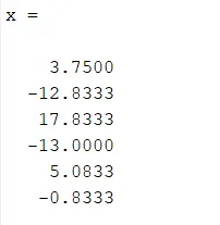
After solving the above matrix , we get the values of coefficients as
a= 3.7500, b= -12.8333, c= 17.8333, d= -13.0000, e= 5.0833, g= -0.8333
Now, dividing both sides of the Hypothesis Eqn.(1) by `(Deltax^2)`; we get,
The Equation using the Taylor table as;
`del^2f/(delx^2)=(af(i)+bf(i-1)+cf(i-2)+df(i-3)+ef(i-4)+gf(i-5))/(Deltax^2)`
Now, from our Taylor table:
`(del^2f)/(delx^2)=(a+b+c+d+e+g)f(i)+(-b-2c-3d-4e-5g)f'(i)Deltax+(0+b/2+4c/2+9d/2+16e/2+25g/2)f''(i)Delta x^2+(0-b/6-8c/6-27d/6-64e/6-125g/6)f'''(i) Delta x^3+(0+b/24+16c/24+81d/24+256e/24+625g/24)f''''(i)Deltax^4+(0-b/120-32c/120-243d/120-1024e/120-3125g/120)f'''''(i)Delta x^5+(0+b/720+64c/720+729d/72+4096e/720+15625g/720)f''''''(i) Deltax^6`
On dividing the above equation by `(Deltax^2)`, we get;
`(del^2f)/(delx^2)=(b/2+2c+9d/2+8e+25g/2)f''(i)+(b/720+64c/720+729d/720+4096e/720+15625g/720)f'''''(i) Delta x^4`
As, we discussed earlier, the `Delta x^4`denotes the truncation error. Here, we can see that order of the truncation error;`[0(Delta x^4)]`is '4'. Since, we know that the order of approximation is defined by the truncation error term. Therefore, we can say that out skewed left-sided difference scheme is of 4th order accurate.
3. Central Difference:
The number of nodes required for the 4th order approximation of a second order derivative using Central difference method can be given by the equation
N = P+Q-1 = 2+4-1=5
where, N is the number of nodes
Q is the order of derivative
P is the order of Approximation.
so, Here we need 5 nodes in order to find the 4th order Approximation of the second-order derivative.
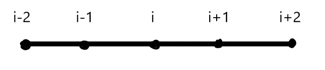
According to the above stencil, The Hypothesis Equation will be,
`del^2f/(del x^2)= af(i-2)+bf(i-1)+cf(i)+df(i+1)+ef(i+2)`
Writing Taylor series Expansion for Hypothesis Equation,
`af(i-2)= af(i)-a(2 Deltax)f'(i)+a(2 Deltax)^2/2.f''(i)-a(2 Delta x)^3/6.f'''(i)+a(2 Delta x)^4/24.f''''(i)-a(2 Delta x)^5/120.f'''''(i)+a(2 Delta x)^6/720.f''''''(i)-...`
`bf(i-1)=bf(i)-b Delta x f'(i)+b Deltax^2/2 f''(i)-b Deltax^3/6 f'''(i)+b Deltax^4/24 f''''(i)-b Deltax^5/120 f'''''(i)+b Deltax^6/720 f''''''(i)-...`
`cf(i)=cf(i)`
`df(i+1)=df(i)+d Delta x f'(i)+d Deltax^2/2 f''(i)+d Deltax^3/6 f'''(i)+d Deltax^4/24 f''''(i)+d Deltax^5/120 f'''''(i)+d Deltax^6/720 f''''''(i)+...`
`ef(i+2)= ef(i)+e(2 Deltax)f'(i)+e(2 Deltax)^2/2.f''(i)+e(2 Delta x)^3/6.f'''(i)+e(2 Delta x)^4/24.f''''(i)+e(2 Delta x)^5/120.f'''''(i)+e(2 Delta x)^6/720.f''''''(i)+...`
Now, Arranging the above taylor series Expansion in taylor table,we get
Consider Taylor table for central difference.
|
Taylor Table |
||||||||
|
Assumed Function |
Taylor Series Expansion |
|||||||
|
`f(i)` |
`Deltax f'(i)` |
`Deltax^2 f''(i)` |
`Deltax^3f'''(i)` |
`Deltax^4 f''''(i)` |
`Deltax^5 f'''''(i)` |
`Deltax^6 f''''''(i)` |
||
|
Stencil |
af(i-2) |
a |
-2a |
4a/2 |
-8a/6 |
16a/24 |
-32a/120 |
64a/720 |
|
bf(i-1) |
b |
-b |
b/2 |
-b/6 |
b/24 |
-b/120 |
b/720 |
|
|
cf(i) |
c |
0 | 0 | 0 | 0 | 0 | 0 | |
|
df(i+1) |
d |
d |
d/2 |
e/6 |
d/24 |
d/120 |
d/720 |
|
|
ef(i+2) |
e |
2e |
4e/2 |
8e/6 |
16e/24 |
32e/120 |
64e/720 |
|
|
Sum of co-efficients `del^2f/(del x^2)` |
0 |
0 |
1 |
0 |
0 |
? |
? |
|
Here, we only considered five terms in our Hypothesis equation, Neglecting the last two terms
Therefore, the five equations are;
`[a+b+c+d+e]=0---(1)`
`[-2a-b+d+2e]=0---(2)`
`[(4a)/2+b/2+d/2+(4e)/2]=1---(3)`
`[(-8a)/6-b/6+d/6+(8e)/6]=0---(4)`
`[(16a)/24+b/24+d/24+(16e)/24]=0---(5)`
Writing the coefficients in the form of a matrix , we get
`[[1,1,1,1,1],[-2,-1,0,1,2],[2,1/2,0,1/2,2],[-8/6,-1/6,0,1/6,8/6],[16/24,1/24,0,1/24,16/24]].[[a],[b],[c],[d],[e]]=[[0],[0],[1],[0],[0]]`
Solving the above matrix form using AX=B in MATLAB to find the values of coefficients
A=[1 1 1 1 1 ;-2 -1 0 1 2;2 1/2 0 1/2 2; -8/6 -1/6 0 1/6 8/6;16/24 1/24 0 1/24 16/24];

B=[0;0;1;0;0];

x=inv(A)*B;
We get,
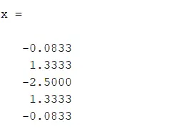
After solving the above matrix , we get the values of coefficients as
a= -0.08333, b= 1.3333, c= -2.5000, d= 1.33333, e= -0.08333
Now, dividing both sides of the Hypothesis Eqn.(1) by `(Deltax^2)`; we get,
The Equation using the Taylor table as;
`del^2f/(delx^2)=(af(i-2)+bf(i-1)+cf(i)+df(i+1)+ef(i+2))/(Deltax^2)`
Program in MATLAB to Evaluate the Second-order Derivative of the analytical function exp(x)*cos(x) and Comparing it with numerical derivative we have derived before:
Firstly, we are going to write programs to develop functions for central, skewed right_sided and skewed_left sided errors at a particular point (x,dx), where dx represents spacing in between each node. These functions will help us to calculate errors over the range of 'dx'. With the help of code 'function out' we're going to make function; which we save in directory and call according to our need in the main program (make sure to save the main program in the same directory in which your function saved).
Function for Skewed-right difference 4th order error at particular spacing 'dx':
% creating function for the 4th order approximation of the second-order
% Derivative using skewed-right sided Difference method

function skewed_right_sided_error=skewed_right_sided_approximation(x,dx)

%Anlaytical function f(x)=exp(x)*cos(x)
%f''(x)=-2*exp(x)*sin(x)

Analytical_derivative=-2*exp(x)*sin(x);

% values of coefficients calculated by solving the matrix form
A=[1 1 1 1 1 1;0 1 2 3 4 5;0 1/2 4/2 9/2 16/2 25/2;0 1/6 8/6 27/6 64/6 125/6;0 1/24 16/24 81/24 256/24 625/24;0 1/120 32/120 243/120 1024/120 3125/120];
B=[0;0;1;0;0;0];
x_r=inv(A)*B;

%numerical derivative
%skewed right-sided differencing=((a*f(x))+(b*f(x+dx))+(c*f(x+2dx))+(d*f(x+3dx))+(e*f(x+4dx))+(g*f(x+5dx)))/(dx^2)
%skewed right-sided fourth order approximation

skewed_right_sided_fourth_order_approx=((x_r(1)*exp(x)*cos(x))+(x_r(2)*exp(x+dx)*cos(x+dx))+(x_r(3)*exp(x+2*dx)*cos(x+2*dx))+(x_r(4)*exp(x+3*dx)*cos(x+3*dx))+(x_r(5)*exp(x+4*dx)*cos(x+4*dx))+(x_r(6)*exp(x+5*dx)*cos(x+5*dx)))/(dx^2);

skewed_right_sided_error=abs(skewed_right_sided_fourth_order_approx-Analytical_derivative);

end
Function for Skewed-left difference 4th order error at particular spacing 'dx':
% creating function for the 4th order approximation of the second-order
% Derivative using skewed-left sided Difference method

function skewed_left_sided_error=skewed_left_sided_approximation(x,dx)

%Anlaytical function f(x)=exp(x)*cos(x)
%f''(x)=-2*exp(x)*sin(x)

Analytical_derivative=-2*exp(x)*sin(x);

% values of coefficients calculated by solving the matrix form
C=[1 1 1 1 1 1;0 -1 -2 -3 -4 -5;0 1/2 4/2 9/2 16/2 25/2;0 -1/6 -8/6 -27/6 -64/6 -125/6;0 1/24 16/24 81/24 256/24 625/24;0 -1/120 -32/120 -243/120 -1024/120 -3125/120];
D=[0;0;1;0;0;0];
x_l=inv(C)*D;

%numerical derivative
%skewed left-sided differencing=((a*f(x))+(b*f(x-dx))+(c*f(x-2dx))+(d*f(x-3dx))+(e*f(x-4dx))+(g*f(x-5dx)))/(dx^2)
%skewed left-sided fourth order approximation

skewed_left_sided_fourth_order_approx=((x_l(1)*exp(x)*cos(x))+(x_l(2)*exp(x-dx)*cos(x-dx))+(x_l(3)*exp(x-2*dx)*cos(x-2*dx))+(x_l(4)*exp(x-3*dx)*cos(x-3*dx))+(x_l(5)*exp(x-4*dx)*cos(x-4*dx))+(x_l(6)*exp(x-5*dx)*cos(x-5*dx)))/(dx^2);

skewed_left_sided_error=abs(skewed_left_sided_fourth_order_approx-Analytical_derivative);

end
Function for Central difference 4th order error at particular spacing 'dx':
% creating function for the 4th order approximation of the second-order
% Derivative using central Difference method

function central_differencing_error=central_differencing_approximation(x,dx)

%Anlaytical function f(x)=exp(x)*cos(x)
%f''(x)=-2*exp(x)*sin(x)

Analytical_derivative=-2*exp(x)*sin(x);

% values of coefficients calculated by solving the matrix form
E=[1 1 1 1 1 ;-2 -1 0 1 2;2 1/2 0 1/2 2; -8/6 -1/6 0 1/6 8/6;16/24 1/24 0 1/24 16/24];
F=[0;0;1;0;0];
x_c=inv(E)*F;

%numerical derivative
%central differencing=((a*f(x-2*dx))+(b*f(x-dx))+(c*f(x))+(d*f(x+dx))+(e*f(x+2*dx)))/(dx^2)
%central differencing fourth order approximation

central_differencing_fourth_order_approx=((x_c(1)*exp(x-2*dx)*cos(x-2*dx))+(x_c(2)*exp(x-dx)*cos(x-dx))+(x_c(3)*exp(x)*cos(x))+(x_c(4)*exp(x+dx)*cos(x+dx))+(x_c(5)*exp(x+2*dx)*cos(x+2*dx)))/(dx^2);

central_differencing_error=abs(central_differencing_fourth_order_approx-Analytical_derivative);

end
Main Program:
%calculating 4th order error of second-order derivative using central,
%skewed right-sided and skewed left-sided differencing method

clear all
close all
clc

x=pi/3;
dx=linspace(pi/4,pi/400,40);

%creating 'for' loop;
for i=1:length(dx)
    central_difference_error(i)=central_differencing_approximation(x,dx(i));
    skewed_right_side_error(i)=skewed_right_sided_approximation(x,dx(i));
    skewed_left_side_error(i)=skewed_left_sided_approximation(x,dx(i));
end

%plotting graphs for dx vs Errors for central, skewed right_sided,
%skewed-left sided Approximations

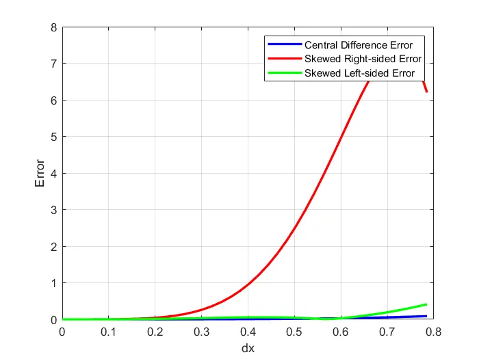
figure(1)
plot(dx,central_difference_error,'linewidth',2)
hold on
grid on
plot(dx,skewed_right_side_error,'r','linewidth',2)
hold on
plot(dx,skewed_left_side_error,'g','linewidth',2)
xlabel('dx')
ylabel('Error')
legend('Central Difference Error','Skewed Right-sided Error','Skewed Left-sided Error')

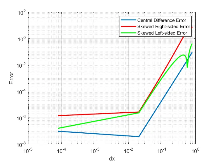
figure(2)
loglog(dx,central_difference_error,'linewidth',2)
hold on
grid on
loglog(dx,skewed_right_side_error,'r','linewidth',2)
hold on
loglog(dx,skewed_left_side_error,'g','linewidth',2)
xlabel('dx')
ylabel('Error')
legend('Central Difference Error','Skewed Right-sided Error','Skewed Left-sided Error')
Graph:
FIGURE(1)
FIGURE(2)
Result:
After analyzing the graph between 'Error' vs. 'dx' for central, skewed righ-sided and skewed left-sided difference 4th order error; we can easily notice that central difference approximation produces more accurate solutions;Hence produces lesser errors as compared to right-skewed and left-skewed difference methods.
Why a skewed scheme is useful? What can a skewed scheme do that a CD scheme cannot do?
A skewed scheme is useful when we have to predict using the boundary condition as we have only one direction to go. Hence the skewed scheme will be useful and we cannot use the central differencing for such an application because it required information from both directions of the point.