Week 11 - Simulation of Flow through a pipe in OpenFoam
Aim
To simulate an axi-symmetric flow by applying the wedge boundary condition and to numerically simulate the Hagen Poiseuille flow through a pipe in OpenFOAM.
Objective
- Writing a program in MATLAB to automate the generation of blockMeshDict file for any wedge angle and grading schemes. It is given that wedge angle should be less than 5 degrees.
- For a baseline mesh, show that the velocity profile matches with the Hagen-Poiseuille Equation.
- To validate Hydro-dynamic length(L_e) with the numerical result.
- To validate the fully developed flow velocity profile with its analytical profile.
- To validate maximum velocity and pressure drop for fully developed flow.
- To show Post-process Shear stress and validate wall shear stress for fully developed flow in Paraview.
Project Methodology
- This project aims to simulate the Hagen-Poiseuille flow throw a pipe of circular cross section, by considering all of the assumptions that were given.
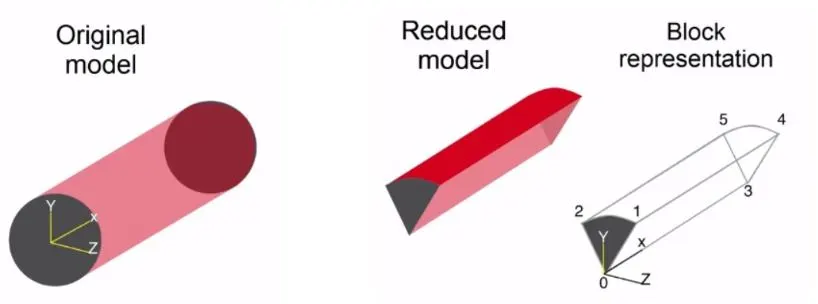
- since the flow is axisymmetric in nature ,a reduced model which is only a section or wedge of the pipe is modelled through which fluid flow is then simulated.
- This is done to reduce the complexity of the problem, and the computational time and resources required enormously.
- The wedge is created by considering a specific wedge angle. A MATLAb script is created to automatically generate the blockmeshdict file by accepting the wedge angle as the input.
- The "icoFoam" solver which is used to solve the incompressible, laminar, Navier Stokes equation is used to simulate the flow through the pipe in this problem.
- The results are then post-processed using ParaView, to observe the velocity profile for the fully developed flow, and at the Hydrodyamic Entrance length of the pipe.
- The variation of shear stress developed along the length of the pipe (axial direction) is also plotted.
- The data from the CFD simulation is validated by comparing against the analytical solutions obtained from the Hagen-Poiseuille Equations to ensure the fidelity of results.
Hagen-Poiseuille flow
The Hagen-Poiseuille flow is a type of fluid flow based on the Hagen-Poiseuille's law, which is a physical law that gives the pressure drop in an incompressible and Newtonian fluid in laminar flow flowing through a long cylindrical pipe of constant pipe of constant cross-section.
The assumptions of the HP equation is that the fluid is incompressible and Newtonian, and the flow is laminar through a pipe of constant cross section, with a length that is sufficiently larger than the diameter of the pipe and that there is no acceleration of the fluid through the pipe.
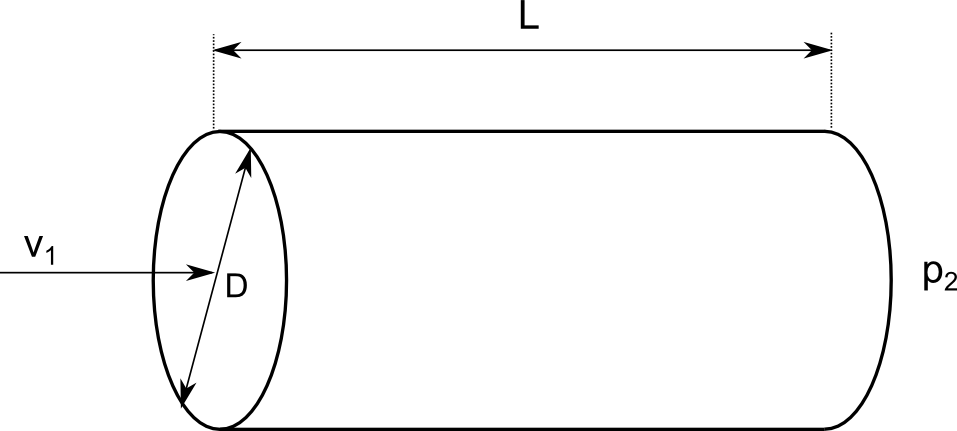
Input Parameters:
- Diameter of the pipe (D)=0.02m
- Wedge Angle `theta`= 4 (should be less then 5)
- Length of the pipe (L) = 3m
- Density of fluid (Water) `rho`= 1000 kg/m^3
- Viscosity of Water at 25 degree celsius = 8.9*10^-4 pa.s
- Reynold's number for Laminar flow (`R_e`) = 2100
The above mentioned input parameters should be considered for deriving the analytical solutions and to generate the blockmeshDict file in MATLAB to be used in OpenFOAM.
Description of Flow Physics
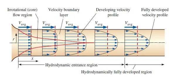
As the working fluid (water in this case) enters the pipe with a constant inlet velocity, the fluid comes in contact with the pipe walls. Because of the no-slip boundary condition, the fluid particles in the layer in contact with the wall come to a complete stop. This layer also causes the fluid particles in the adjacent layers to slow down gradually due to friciton between the layers (fluid viscosity). To make up for this velocity reduction, the velocity of the fluid at the mid-section of the pipe has to increase so that the mass flow rate through the pipe remains constant. As a result of this, a velocity gradient develops along the axial direction or length of the pipe.
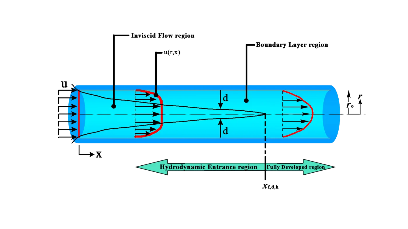
The region of flow in which the effects of viscous shearing forces caused by the fluid viscosity are significantly felt is called the velocity boundary layer or simply the boundary layer. The boundary surface divides the flow in a pipe into two regions: the boundary layer region, in which the viscous effects and velocity changes are significant, and the irrotational (core) flow region (or) the inviscid flow region, in which the friction effects are negligible and the velocity essentially remains constant in the radial direction.
The thickness of the boundary layer gradually increases in the flow direction, until it reaches the mid-section of the pipe, at which point it fills the entire pipe, and the velocity profile becomes fully developed. The region of the pipe from the pipe inlet, to the point at which the flow becomes fully developed is called as the hydrodynamic entrance region, and the length of this region is called the hydrodynamic entrance length (`L_e`).
The flow in this region is called hydrodynamically developing flow since this is the region where the velocity profile develops and keeps changing. The region beyond the entrance region in which the velocity profile is fully developed and remains unchanged across the length of the pipe, is called the hydrodynamically fully developed region. The flow in this region is said to be a fully developed flow and remains constant across the pipe. The velocity profile in the fully developed region is parabolic for laminar flow as shown in the figure below.
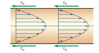
`tau_w`- wall shear stress
Hydrodynamicallly fully devloped flow:
`(delU_(r,x))/(delx) = 0`
`U = U(r)`
Hydrodynamic Entrance length:

where, `L_e= 0.05*Re*D` for Laminar flow
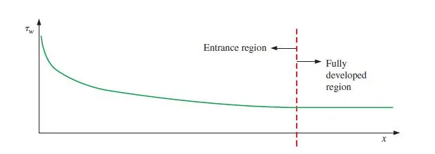
We know that for Newtonian fluids, the shear stress is directly proportional to the veloicty gradient. Thus, the shear stree at the pipe wall (`tau_w`) is also related to the slope of the velocity profile. Since the velocity profile remains unchanged in the fully developed region, the wall shear stress also remains constant in this region. Also, the wall shear stress is highest at the inlet where the thickness of the boundary layer is the smallest, and decreases gradually to the fully developed value as shown in the below figure.
The pressure drop equation of the Hagen poiseuille's is as follows;
`DeltaP = (32muLV_(avg))/(D^2)`
where, `DeltaP = P_1-P_2`
From the above equation, it is clear that the pressure drop across the pipe is directly proportional to the viscosity of the fluid flowing through the pipe. If there were no viscosity (i.e, no friction), the pressure loss would be Zero. Hence, the pressure drop in the above case is entirely due to the fluid viscosity.
Deriving Analytical solutions for Flow parameters from Hagen-Poiseuille's Equation
In order to validate the CFD results obtained, and to ensure their fidelity, they should be compared with analytically obtained values. These analytical values are obtained through different analytical equations, describing different flow parameters.
1. Reynold's Number, `Re = (rhoV_(avg)D)/(mu)`
`2100 = (1000*V_(avg)*0.02)/(8.92xx10^-4)`
`therefore``V_(avg) = 0.0937`m/s
2. Maximum Velocity at Centre line;
`V_max = 2*V_(avg)`
`V_max=> 2*0.0937 = 0.1875m/s`
3. Hydrodynamic Entrance Length;
`L_e= 0.05xxDxxRe = 0.05xx0.02xx2100 = 2.1m`
4. Pressure drop across the pipe from HP Equation:
`Delta p = (32muLV_(avg))/(D^2) = (32xx8.9xx10^-4xx3xx0.0937)/(0.02^2) = 20.014 Pa`
5. Kinematic Pressure drop
`DeltaP_k = (DeltaP)/(rho) = 20.014/1000 = 0.020Pa`
6. Velocity Profile at any location in the fully devloped region ;
`U(r) = 2*V_(avg)*(1-(r^2)/(R^2))`
Where, 'r ' represents the radial distance from the centre of the pipe.
The analytical values and equations described above will be used for comparing against the CFD results to ensure their validity. A MATLAB Script is written to evaluate these values for the flow parameters, and to generate the computational mesh automatically through the blockMeshDict file for usage in OpenFOAM.
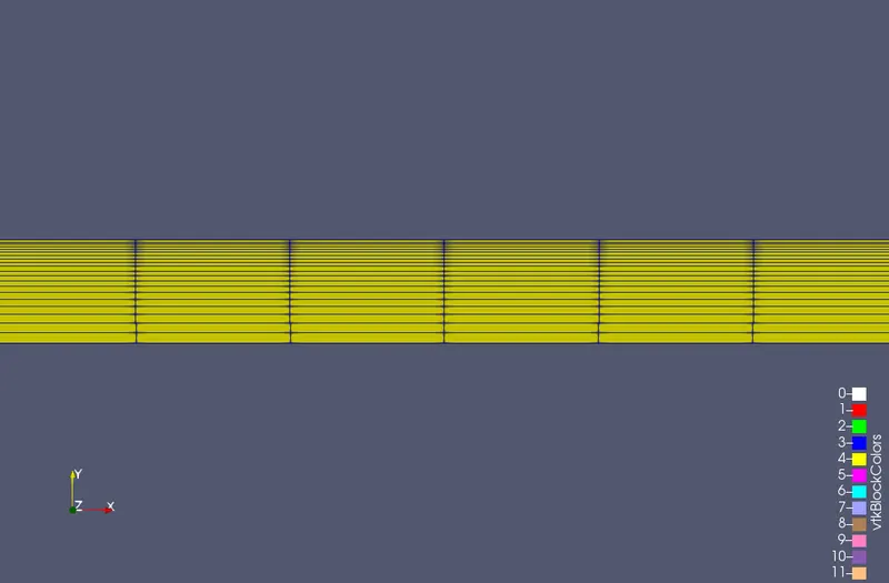
The Geometry under consideration for fluid flow simulation is a reduced model that has been designed to ensure minimal use of computational resources. This geometry is shown in the figure below. Since the geometry of the pipe is axisymmetric along the x axis, a section of the pipe is modelled and the boundary conditions are provided accordingly. Also, since it is essential to capture the boundary layer developed at the topwall of the wedge, a grading factor is given to the mesh to obtain a locally refined mesh. This locally refined mesh is used to sufficiently model and capture the boundary layer developed during the fluid flow, and to determine the velocity profile developed during the flow.
MATLAB Code
clear all
close all
clc

%Blockmesh file for simulating flow through apipe

%Reynolds number for laminar flow
Re=2100;
%Density of Water
rho=1000; %unit kg/m^3
% Dynamic Viscosity of Water
mu=8.9e-4;
%diameter of the pipe
D=0.02;
%Radius of the pipe
R=D/2;
%Hydrodynamic Entrance length of the pipe
L_e= 0.05*D*Re;
L =3; % Total Length of the pipe

% Caculating Average velocity from Reynold's Number
v_avg = (Re*mu)/(rho*D);
% Maximum velocity at the centre of the pipe
v_max = 2*v_avg;
% Calculating Pressure drop from Hagen Poiseuille's equation
delta_p = (32*mu*L*v_avg)/(D^2);
% kinetic pressure drop
delta_p_k = (delta_p)/rho;

% Input the wedge angle should be less than 5 degree
theta = input('Enter the wedge angle = ');

%Mesh parameters
%No.of mesh points
mesh_x = 200;
mesh_y = 20;
mesh_z = 1;
%Mesh grading factors
grade_x = 1;
grade_y = 0.2;
grade_z = 1;

% Determining the vertices of the wedge
% where y=d/2*cosd(theta/2) and z=d/2*sind(theta/2)
v0=[0,0,0];
v1=[0,(R*cosd(theta/2)),(R*sind(theta/2))];
v2=[0,(R*cosd(theta/2)),(-R*sind(theta/2))];
v3=[L,0,0];
v4=[L,(R*cosd(theta/2)),(R*sind(theta/2))];
v5=[L,(R*cosd(theta/2)),(-R*sind(theta/2))];

%Parsing blockMeshDict file
f1=fopen('blockMeshDict.txt','w');
fprintf(f1,'%s','/*--------------------------------*- C++ -*----------------------------------*');
fprintf(f1,'n=========                 |');
fprintf(f1,'n      /  F ield         | OpenFOAM: The Open Source CFD Toolbox');
fprintf(f1,'n    /   O peration     | Website:  https://openfoam.org');
fprintf(f1,'n  /    A nd           | Version:  8');
fprintf(f1,'n/     M anipulation  |');
fprintf(f1,'n%s','*---------------------------------------------------------------------------*/');
fprintf(f1,'nFoamFile');
fprintf(f1,'n{');
fprintf(f1,'nversion     2.0;');
fprintf(f1,'nformat      ascii;');
fprintf(f1,'nclass       dictionary;');
fprintf(f1,'nobject      blockMeshDict;');
fprintf(f1,'n}');
fprintf(f1,'n%s','// * * * * * * * * * * * * * * * * * * * * * * * * * * * * * * * * * * * * * //');
fprintf(f1,'nnconvertToMeters 1;');

%Creating the vertices
fprintf(f1,'nnvertices');
fprintf(f1,'n(');
fprintf(f1,'nt(%f %f %f)ttt//point0',v0(1),v0(2),v0(3));
fprintf(f1,'nt(%f %f %f)ttt//point1',v1(1),v1(2),v1(3));
fprintf(f1,'nt(%f %f %f)ttt//point2',v2(1),v2(2),v2(3));
fprintf(f1,'nt(%f %f %f)ttt//point3',v3(1),v3(2),v3(3));
fprintf(f1,'nt(%f %f %f)ttt//point4',v4(1),v4(2),v4(3));
fprintf(f1,'nt(%f %f %f)ttt//point5',v5(1),v5(2),v5(3));
fprintf(f1,'n);');

% Block mesh generation
fprintf(f1,'nnblocks');
fprintf(f1,'n(');
fprintf(f1,'nt hex (0 3 5 2 0 3 4 1) (%d %d %d) simpleGrading (%f %f %f)',mesh_x,mesh_y,mesh_z,grade_x,grade_y,grade_z);
fprintf(f1,'n);');

%edges arc formation
fprintf(f1,'nn edges');
fprintf(f1,'n(');
fprintf(f1,'nt arc 1 2 (%f %f %f)',0,R,0);
fprintf(f1,'nt arc 4 5 (% f %f %f)',L,R,0);
fprintf(f1,'n);');

%Boundary conditions formation
fprintf(f1,'nnboundary');
fprintf(f1,'n(');
fprintf(f1,'ntinlet nt{');
fprintf(f1,'ntttype patch;');
fprintf(f1,'nttfaces');
fprintf(f1,'ntt(');
fprintf(f1,'ntt(0 1 2 0)');
fprintf(f1,'ntt);');
fprintf(f1,'nt}');
fprintf(f1,'ntoutlet nt{');
fprintf(f1,'ntttype patch;');
fprintf(f1,'nttfaces');
fprintf(f1,'ntt(');
fprintf(f1,'ntt(3 4 5 3)');
fprintf(f1,'ntt);');
fprintf(f1,'nt}');
fprintf(f1,'nttopwall nt{');
fprintf(f1,'ntttype wall;');
fprintf(f1,'nttfaces');
fprintf(f1,'ntt(');
fprintf(f1,'ntt(1 2 5 4)');
fprintf(f1,'ntt);');
fprintf(f1,'nt}');
fprintf(f1,'ntfront nt{');
fprintf(f1,'ntttype wedge;');
fprintf(f1,'nttfaces');
fprintf(f1,'ntt(');
fprintf(f1,'ntt(0 1 4 3)');
fprintf(f1,'ntt);');
fprintf(f1,'nt}');
fprintf(f1,'ntback nt{');
fprintf(f1,'ntttype wedge;');
fprintf(f1,'nttfaces');
fprintf(f1,'ntt(');
fprintf(f1,'ntt(0 3 5 2)');
fprintf(f1,'ntt);');
fprintf(f1,'nt}');
fprintf(f1,'nt axis nt{');
fprintf(f1,'ntttype empty;');
fprintf(f1,'nttfaces');
fprintf(f1,'ntt(');
fprintf(f1,'ntt(0 3 3 0)');
fprintf(f1,'ntt);');
fprintf(f1,'nt}');
fprintf(f1,'n);');

%mergepatch pairs
fprintf(f1,'nnmergePatchPairs');
fprintf(f1,'n(');
fprintf(f1,'n);');
fprintf(f1,'nn%s','// ************************************************************************* //');
The code used above generates a blockMeshDict text file that is used by OpenFOAM to create the geometry of the pipe as the Wedge with the computational mesh. The blockMeshDict file generated by the above code is attached below.
BlockMeshDict file
/*--------------------------------*- C++ -*----------------------------------*
=========                 |
      /  F ield         | OpenFOAM: The Open Source CFD Toolbox
    /   O peration     | Website:  https://openfoam.org
  /    A nd           | Version:  8
/     M anipulation  |
*---------------------------------------------------------------------------*/
FoamFile
{
version     2.0;
format      ascii;
class       dictionary;
object      blockMeshDict;
}
// * * * * * * * * * * * * * * * * * * * * * * * * * * * * * * * * * * * * * //

convertToMeters 1;

vertices
(
	(0.000000 0.000000 0.000000)			//point0
	(0.000000 0.009994 0.000349)			//point1
	(0.000000 0.009994 -0.000349)			//point2
	(3.000000 0.000000 0.000000)			//point3
	(3.000000 0.009994 0.000349)			//point4
	(3.000000 0.009994 -0.000349)			//point5
);

blocks
(
	 hex (0 3 5 2 0 3 4 1) (200 20 1) simpleGrading (1.000000 0.200000 1.000000)
);

 edges
(
	 arc 1 2 (0.000000 0.010000 0.000000)
	 arc 4 5 ( 3.000000 0.010000 0.000000)
);

boundary
(
	inlet
	{
		type patch;
		faces
		(
		(0 1 2 0)
		);
	}
	outlet
	{
		type patch;
		faces
		(
		(3 4 5 3)
		);
	}
	topwall
	{
		type wall;
		faces
		(
		(1 2 5 4)
		);
	}
	front
	{
		type wedge;
		faces
		(
		(0 1 4 3)
		);
	}
	back
	{
	        type wedge;
	        faces
	        (
	        (0 3 5 2)
	        );
	}
	 axis
	{
		type empty;
		faces
		(
		(0 3 3 0)
		);
	}
);

mergePatchPairs
(
);

// ************************************************************************* //
The command 'blockMesh'is used to execute the blockMeshDict file and it will generate the automated mesh. 'checkMesh' is used to check the mesh and to confirm 'Mesh ok'.
Initial Conditions
The initial conditions for pressure and velocity for the timestep 0 are described in the '0' directory in OpenFOAM.
Velocity file
/*--------------------------------*- C++ -*----------------------------------*
  =========                 |
        /  F ield         | OpenFOAM: The Open Source CFD Toolbox
       /   O peration     | Website:  https://openfoam.org
      /    A nd           | Version:  8
     /     M anipulation  |
*---------------------------------------------------------------------------*/
FoamFile
{
    version     2.0;
    format      ascii;
    class       volVectorField;
    object      U;
}
// * * * * * * * * * * * * * * * * * * * * * * * * * * * * * * * * * * * * * //

dimensions      [0 1 -1 0 0 0 0];

internalField   uniform (0 0 0);

boundaryField
{
    inlet
    {
        type            fixedValue;
        value           uniform (0.0937 0 0);
    }

    outlet
    {
        type            zeroGradient;
    }

    front
    {
        type            wedge;
    }

    back
    {
        type            wedge;
    }

    topwall
    {
        type            noSlip;
    }

    axis
    {
        type            empty;
    }
}

// ************************************************************************* //
Pressure file
Here, the outlet pressure is given as 0, and the inlet pressure is given as zeroGradient, to calculate the pressure drop across the pipe.
/*--------------------------------*- C++ -*----------------------------------*
  =========                 |
        /  F ield         | OpenFOAM: The Open Source CFD Toolbox
       /   O peration     | Website:  https://openfoam.org
      /    A nd           | Version:  8
     /     M anipulation  |
*---------------------------------------------------------------------------*/
FoamFile
{
    version     2.0;
    format      ascii;
    class       volScalarField;
    object      p;
}
// * * * * * * * * * * * * * * * * * * * * * * * * * * * * * * * * * * * * * //

dimensions      [0 2 -2 0 0 0 0];

internalField   uniform 0;

boundaryField
{
    inlet
    {
        type            zeroGradient;
    }

    outlet
    {
        type            fixedValue;
        value           uniform 0
    }

    topwall
    {
        type            zeroGradient;
    }

    front
    {
        type            wedge;
    }

    back
    {
        type            wedge;
    }

    axis
    {
        type            empty;
    }
}

// ************************************************************************* //
ControlDict file - Specifying Time Step Value
The time-step value for the simulation is determined by the CFL Criterion, given below.
`CFL = (U_max*dt)/(dx)`
Time step `DeltaT`=0.01s
End time = 50s
In order to ensure that the fluid flow completely covers the pipe and attains a steady-state value, a sufficient amount of time must be provided.
/*--------------------------------*- C++ -*----------------------------------*
  =========                 |
        /  F ield         | OpenFOAM: The Open Source CFD Toolbox
       /   O peration     | Website:  https://openfoam.org
      /    A nd           | Version:  8
     /     M anipulation  |
*---------------------------------------------------------------------------*/
FoamFile
{
    version     2.0;
    format      ascii;
    class       dictionary;
    location    "system";
    object      controlDict;
}
// * * * * * * * * * * * * * * * * * * * * * * * * * * * * * * * * * * * * * //

application     icoFoam;

startFrom       startTime;

startTime       0;

stopAt          endTime;

endTime         50;

deltaT          0.01;

writeControl    timeStep;

writeInterval   20;

purgeWrite      0;

writeFormat     ascii;

writePrecision  6;

writeCompression off;

timeFormat      general;

timePrecision   6;

runTimeModifiable true;


// ************************************************************************* //
transportProperties file
/*--------------------------------*- C++ -*----------------------------------*
  =========                 |
        /  F ield         | OpenFOAM: The Open Source CFD Toolbox
       /   O peration     | Website:  https://openfoam.org
      /    A nd           | Version:  8
     /     M anipulation  |
*---------------------------------------------------------------------------*/
FoamFile
{
    version     2.0;
    format      ascii;
    class       dictionary;
    location    "constant";
    object      transportProperties;
}
// * * * * * * * * * * * * * * * * * * * * * * * * * * * * * * * * * * * * * //

nu              [0 2 -1 0 0 0 0] 1e-6;


// ************************************************************************* //
Simulation of Fluid flow using Solver 'icoFoam'
- Once the physical problem has been set up with the appropriate initial and boundary conditions, the problem setup should be solved using the solvers provided in OpenFOAM. The solver used for simulating the flow is selected depending upon the type of problem to be solved.
- In this case, since the Hagen-Poiseuille Flow is the flow to be simulated, the characteristics of the Hagen-Poiseuille Flow should align with the solver characteristics. Since Hagen-Poiseuille Flow is an incompressible, Newtonian, and Laminar Flow, the incompressible solver icoFoam is used to simulate the flow phenomena. icoFoam solves the incompressible laminar Navier-Stokes equations using the PISO algorithm.
- The code is inherently transient, requiring an initial condition (such as zero velocity) and boundary conditions. The icoFOAM code can take mesh non-orthogonality into account with successive non-orthogonality iterations. The number of PISO corrections and non-orthogonality corrections are controlled through user input.
Post-Processing using ParaFoam
The Post-Processing of results is done using 'ParaView', using 'paraFoam' command will open the paraView.
Mesh
Velocity at Inlet
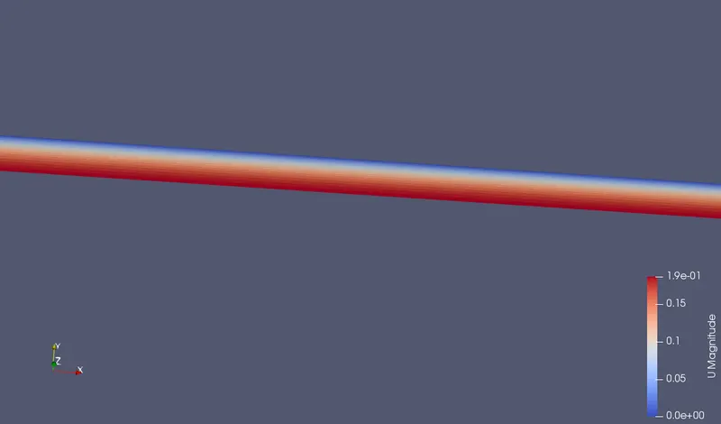
Velocity Distribution along the pipe
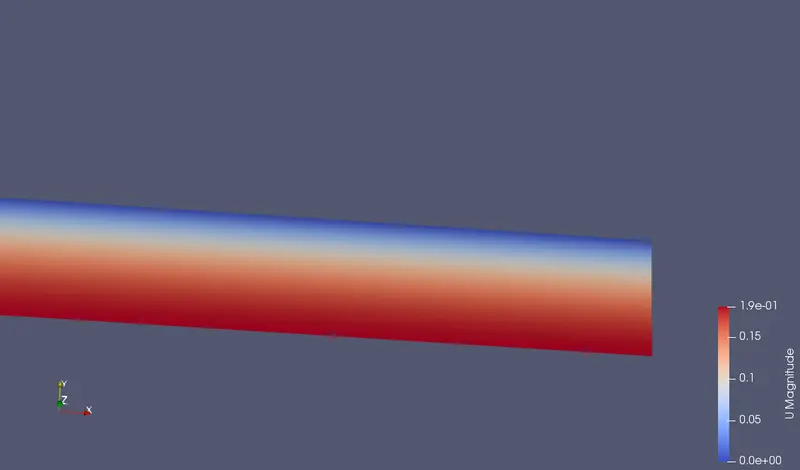
Velocity at Outlet
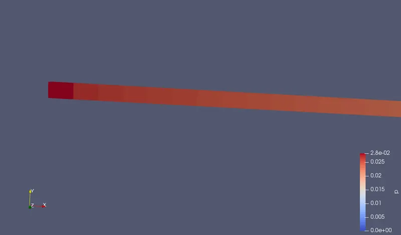
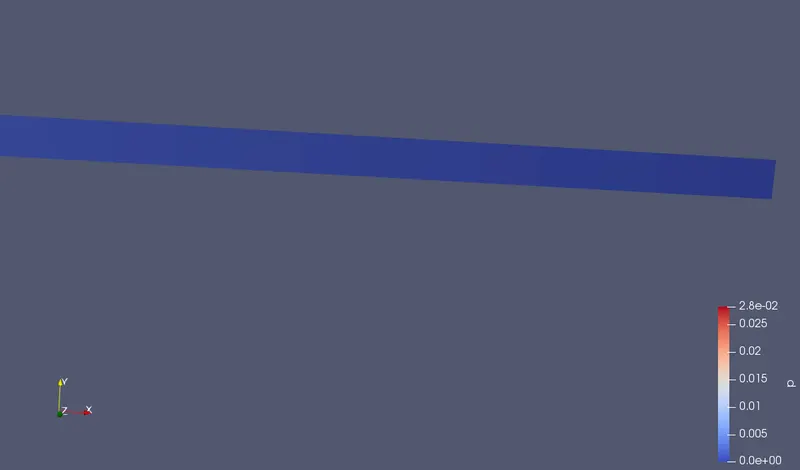
Pressure at Inlet
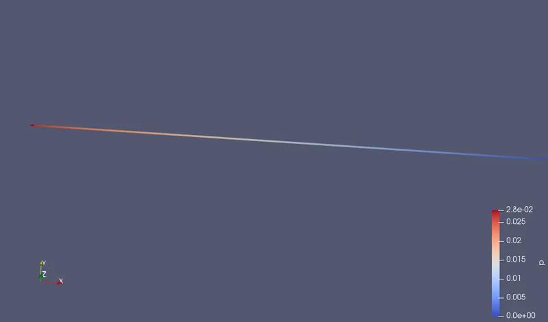
Pressure distribution along the pipe
Pressure at Outlet
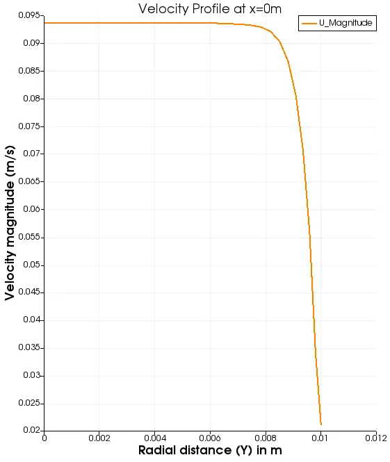
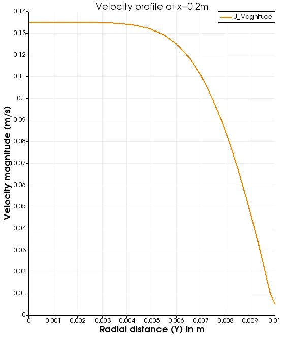
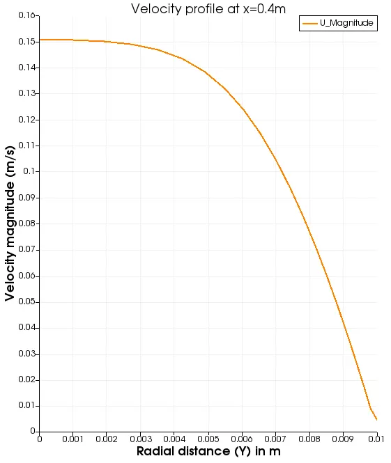
Plot of Velocity Distribution along the Radial Distance at different points along the Pipe Length
Velocity profile at x=0m (inlet)
Velocity Profile at x=0.2m
velocity profile at x=0.4m
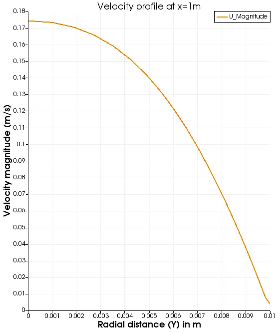
Velocity Profile at x=1m
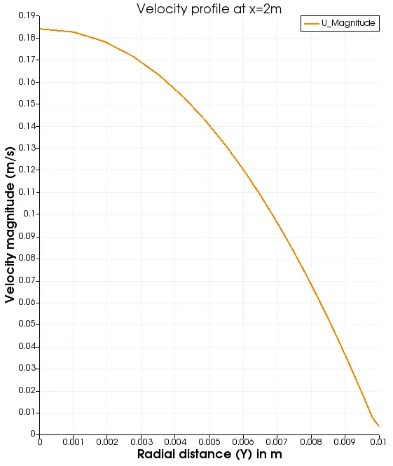
Velocity Profile at x=2m
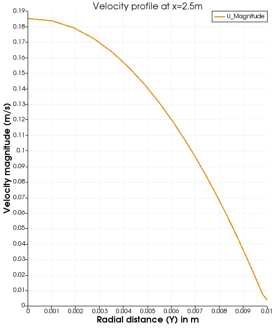
Velocity Profile at x=2.5m
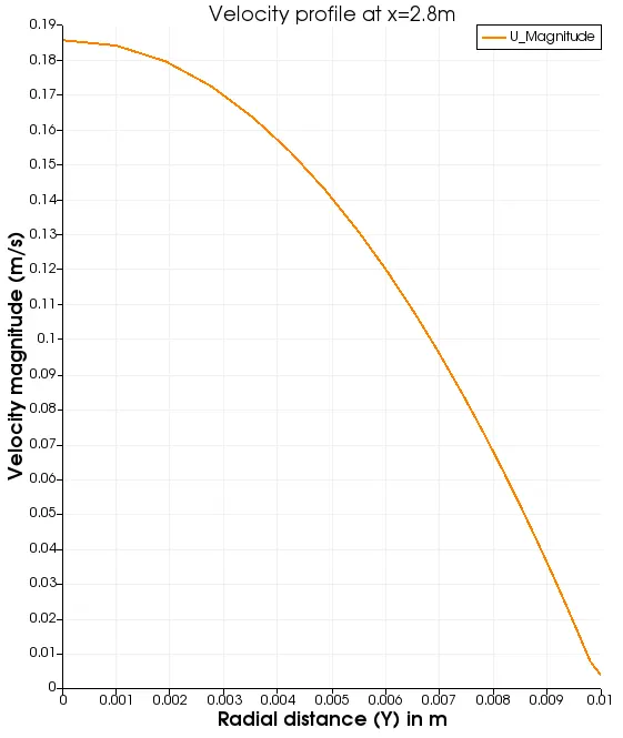
Velocity Profile at x=2.8m
Velocity profile at x=3m
Velocity along the pipe
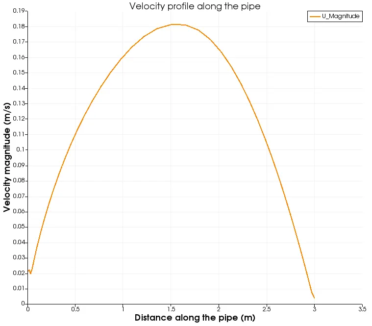
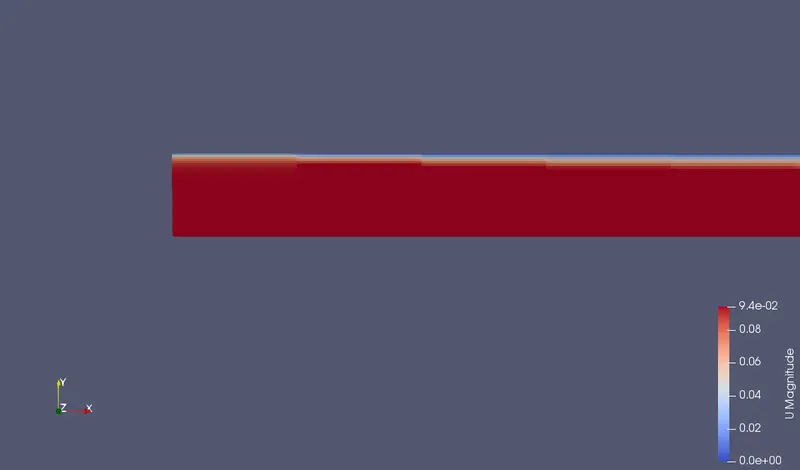
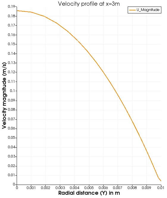
- From the above plots, it is clear that as the fluid enters the pipe with a constant velocity of `V_(avg)`=0.0937m/s at x=0m and progresses through the pipe, the velocity profile along the radial distance keeps changing.
- As the fluid approaches the hydrodynamically fully developed region, the velocity profile becomes progressively more parabolic, and the maximum velocity of the fluid also keeps increasing at x=0.2,0,4,1,and 2m.
- The hydrodynamic entrance length of the flow is `L_e`=2.1m
- After the fluid crosses this length, the flow becomes fully developed and reamins constant throughout the remaining length of the pipe.
- Thus, at the point x=2.8m and x=3m , the flow is fully developed and the velocity profile is completely parabolic, as can be seen in the last two plots shown above. The maximum velocity obtained from the plots in the fully developed region is given as `V_max`=0.1855 m/s.
Plot of Pressure distribution along the pipe Length
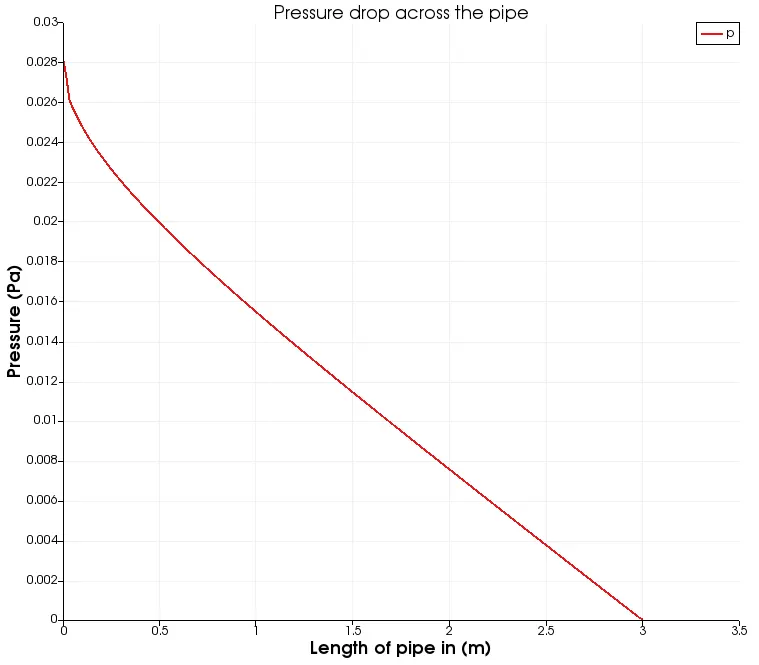
- The above plot shows the pressure drop across the length of the pipe. The pressure at outlet was given as 0 Pa and the pressure at inlet from the plot is shown to be 0.028Pa.
- Thus the pressure drop across the pipe from CFD data, can be calculated as,
`DeltaP=P_1-P_2= 0.028-0 = 0.028Pa`
Plot Of Wall Shear stress distribution along the Radial distance at x=3m
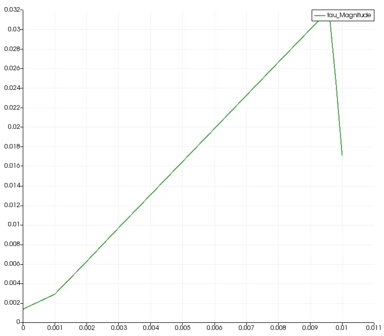
- The above plot shows the variation of shear stress along the radial distance (y axis) of the pipe at x=3m (fully developed flow region)
- In the hydrodynamically fully developed flow regime, the wall shear stress varies linearly from the centre of the pipe (i.e. r=0) to the pipe walls (r=0.01m)
- The wall shear stress value reaches a maximum approximately near the pipe walls.
- This distribution is in agreement with the analytical results, which states that the wall shear stress produced during the flow is directly proportional to the velocity gradient along the Y axis.(i.e.. `tau = mu(delu)/(dely)`)
- The maximum shear stress obtained from the plot is given as, `tau_(max)=0.032Pa`
Comparison of Analytical results vs CFD results for Velocity profile along the radial distance
| Flow Parameter | CFD Value | Analytical Value | % Error |
| Maximum Velocity along Radial Distance | 0.1855 m/s | 0.1875 m/s | 1.06% |
From the table above, it is clear that the obtained CFD solution is in close agreement with the analytical solution. Hence, the validity of the reduced model (i.e Wedge) has been successfully done.
Conclusion:
- The Hagen-Poiseuille flow was computationally simulated successfully and the results are found to be in good agreement with the analytical values derived from the Hagen-Poiseuille Equations.
- The Hagen-Poiseuille Flow was simulated by using a reduced model in the form of a wedge with a specific angle, instead of a fully cylindrical pipe with circular cross-section. This was done to reduce the amount of computational time and resources required to simulate the flow.
- The CFD results obtained for the reduced model were found to be in good agreement with the analytical results, hence confirming the validity of the reduced model as a replacement for the full pipe geometry.
- The wall shear stress distribution along the radial distance of the pipe was found and the maximum wall shear stress obtained from the CFD Results was similar to the theoretical maximum, calculated from analytical equations.
- The pressure drop across the pipe due to the viscosity of the fluid, obtained from CFD Results, was also found to be in good agreement with the result obtained from the Hagen-Poiseuille Equation.
- Hence, it can be concluded that the CFD simulation with correct assumptions and approximations yields results similar to and in close agreement with results obtained from close-form analytical equations.