Week 4 - CHT Analysis on Exhaust port

AIM: To simulate Conjugate Heat Transfer Analysis on the Exhaust port.

OBJECTIVES:

1. Give a brief description of why and where a CHT analysis is used.
2. Maintain the y+ value according to the turbulence model and justify the results.
3. Calculate the wall/surface heat transfer coefficient on the internal solid surface & show the velocity & temperature contours in appropriate areas.
4. How would you verify if the HTC predictions from the simulation are right? On what factors does the accuracy of the prediction depend?

THEORY:

Conjugate Heat Transfer

The key element in having a conjugate heat transfer, as the name suggests the thermal interaction between a fluid and a solid region. This is the basic and most important element of a conjugate heat transfer simulation. If we want to divide it, Into solid regions we are simulating the heat conduction, heat conduction is basically the diffusion of heat due to direct contact. In the fluid regions, we are dealing with Convection of heat, this is the kind of transfer of thermal energy due to the movement of fluid elements. At the interfaces between these two regions, we have the thermal coupling that's why the name is Conjugate heat transfer because we are considering the transfer of mass and thermal energy at the same time both in solid and fluid.

Advantages:

Conjugate Heat Transfer has many advantages that's why it is used.

• Accurate and fast
• Suited for complex scenarios
• Assemblies: no limits on the number of regions
• All types of region combinations like solid-fluid, fluid-fluid can be simulated.

Applications of CHT:

• Cooling of electronic devices
• Heat exchangers
• HVAC

- Heating

- Ventilating

- Air conditioning

• Combustors and Burners
• Gas turbine design
• Engine cooling
• Home appliances
• ...

CONJUGATE HEAT TRANSFER ANALYSIS ON THE EXHAUST PORT:

We will be using the made-up geometry but it contains all the features that the actual exhaust port would have. The exhaust port is a three-dimensional model containing four inlets and one outlet. Our objective is to simulate the flow through it. The flow is going through the manifold and exchanges heat with the solid we want to simulate that process. We are going to assume initially that the flow that is coming through exhaust which is basically all these four inlets and that fluid is really hot and that is going to heat the solid pipe from inside. On the external surface, we are assuming the particular heat transfer coefficient. Air near the exhaust port has a particular heat transfer coefficient that would be provided as the input.

The steps used for solving the problem:

Geometry:

1. Loaded the Exhaust port model into the SpaceClaim and changed the units to meters.

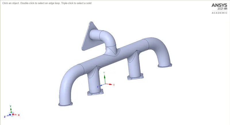
2. Extracted the volume and named the inner volume as fluid volume and outer volume as the solid volume.

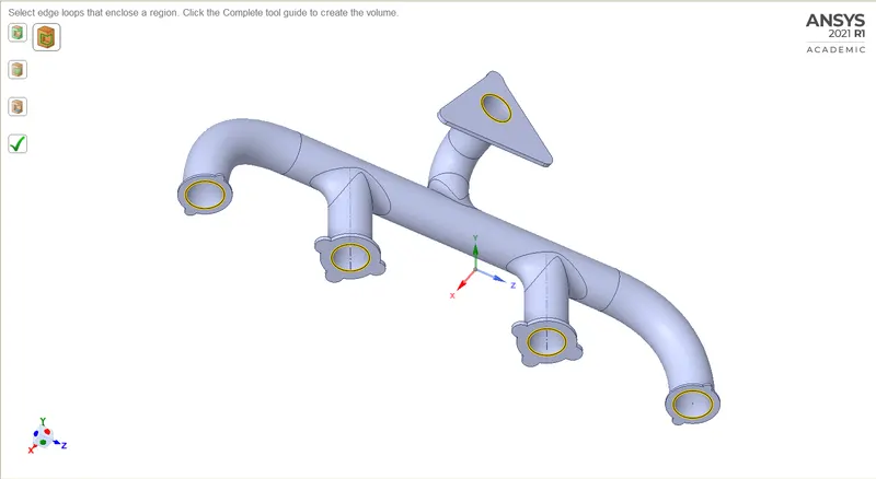
Fluid Volume

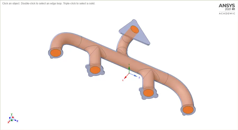
Solid Volume

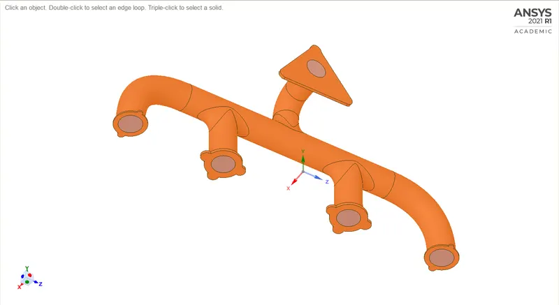
3. The solid and liquid volumes are copied into one component i.e. final component and deleted the empty components.

4. Enabled share topology of the main component so that the mesh and physics information can be shared and conformal mesh can be achieved.

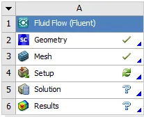
5. To achieve conjugate heat transfer between the fluid and the solid wall we had to choose the share option under the workbench tool this is very important if it is not done we will not see the interfaces where information is being shared so this is very important if we don't do this step and directly go to the meshing interface the mesh will definitely fail. Basically, this particular step takes care of creating the interfaces so that we have one interface between the solid block and fluid block.

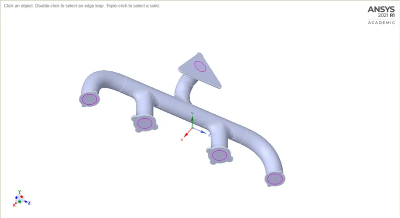
We can see these pink circles that basically tell us where information is being shared.

Mesh:

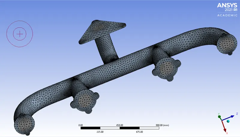
1. After the geometry setup opened the Mesh.

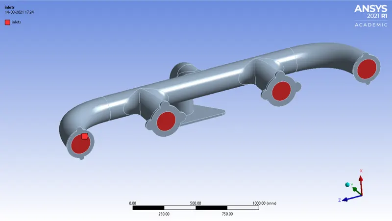
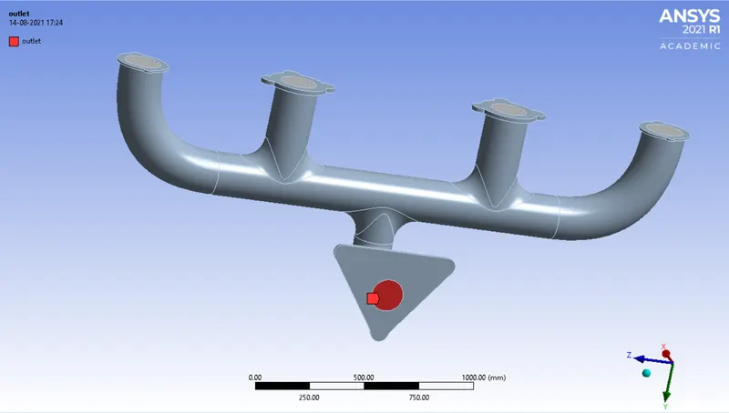
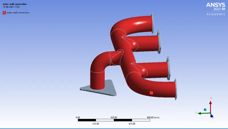
2. Selected the faces and named them.

Inlets

Outlet

Outer wall convection

Baseline Mesh:

Setup:

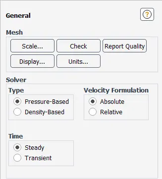
1. After meshing opened the fluent Setup, In the general setting selected a pressure-based solver, steady-state time simulation, absolute velocity formulation, and enabled energy option.

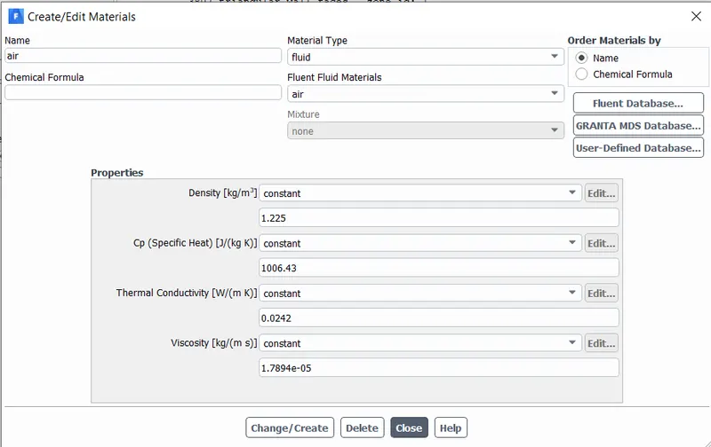
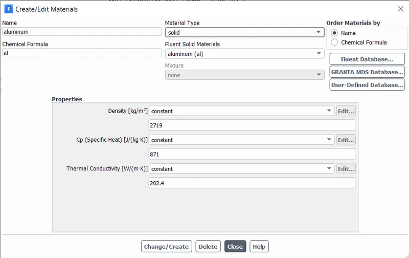
2. Materials >

3. Boundaries >

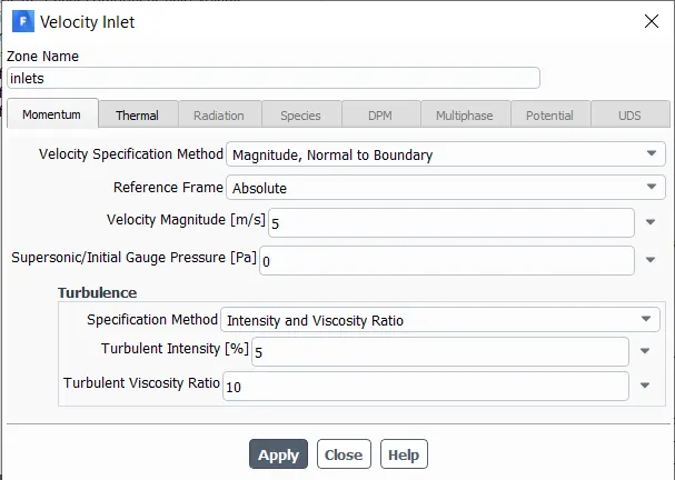
Velocity inlet : `5 m/sec`

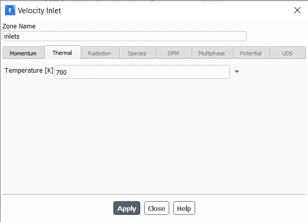
Temperature: `700 k`

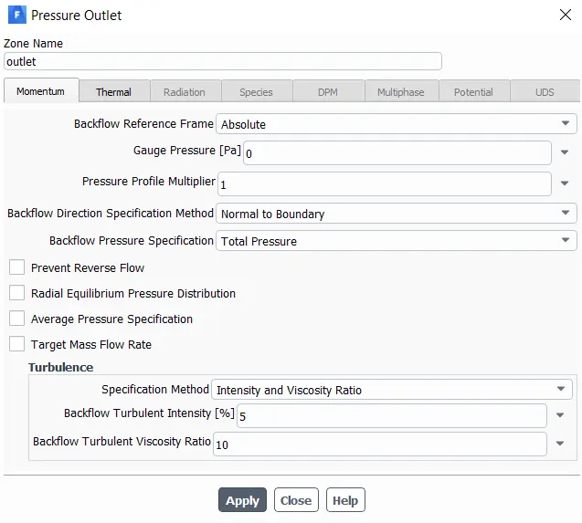
Pressure outlet: gauge pressure = `0 pa`

Outer wall convection:

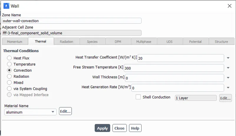
The rest boundary condition values are set up as default values.

4. Reference values >

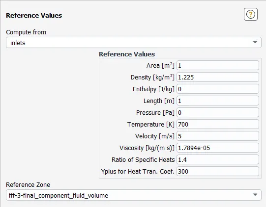
5. Viscous model >

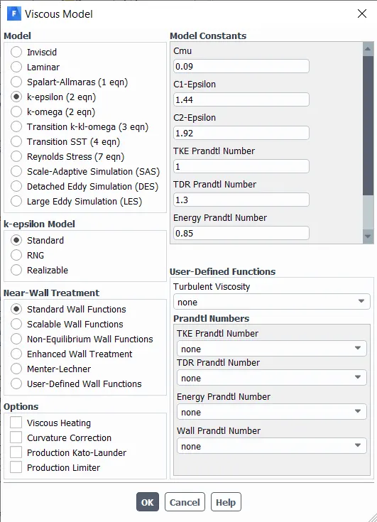
Results:

Residual plot:

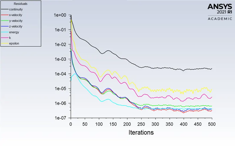
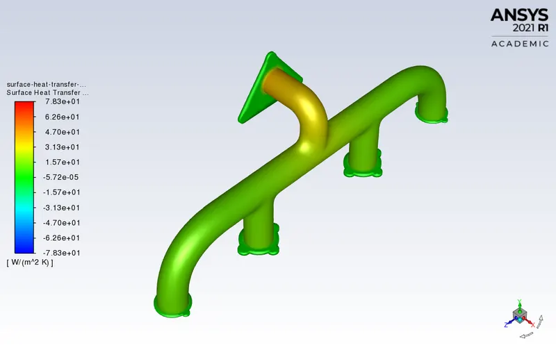
Surface heat transfer coefficient:

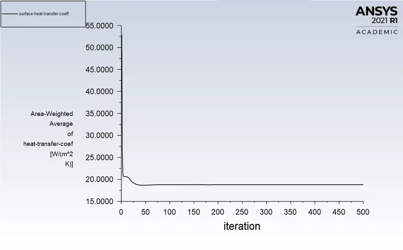
Surface heat transfer coefficient value = 18.793322

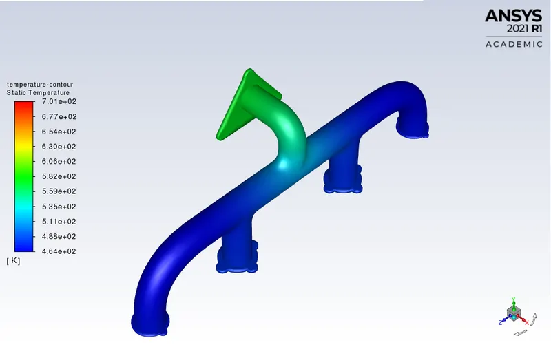
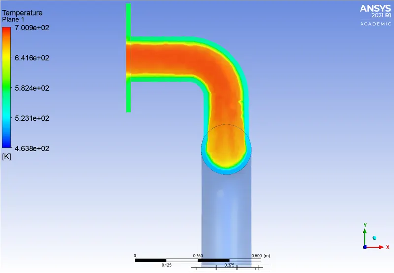
Temperature:

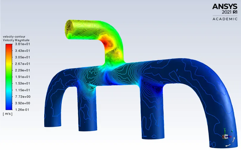
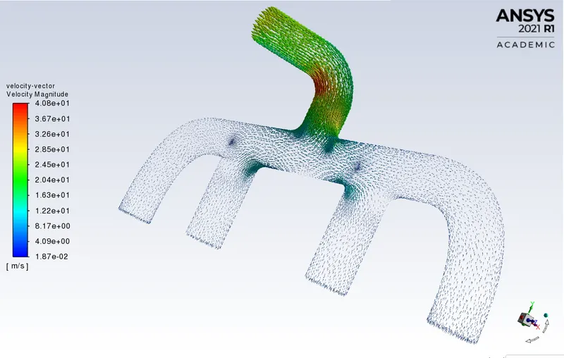
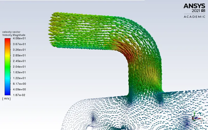
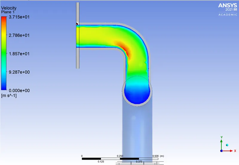
Velocity:

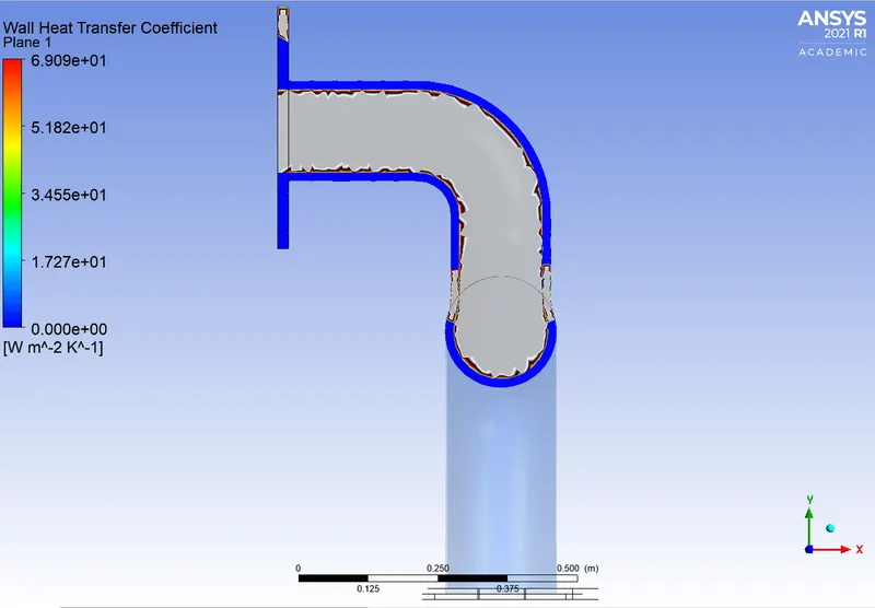
Heat transfer coefficient:

Analytical solution:

Density `rho = 1.225 (kg)/m^3`

Spercific heat `C_p = 1006.43 J/(kg K)`

Thermal conductivity `k = 0.0242 W/(m K)`

Viscosity `mu = 0.000017894 (kg)/(m s)`

Velocity `v = 5 m/s`

Diameter `D = 0.16611 m`

Reynolds number `Re = (rho*v*D)/(mu)`

`= 56858.37`

Nusselt number `Nu = 0.023*Re^(0.8)*Pr^(0.3)`

Prandtl number `Pr = (mu*C_p)/(k)`

`= (0.000017894*1006.43)/(0.0242)`

`= 0.74`

Then Nusselt number `Nu = 0.023*(56858.37)^0.8*(0.74)^0.3`

`= 133.76`

The Nusselt number can also be written as `Nu = (h*D)/(k)`

where h = heat transfer coefficient, `h = (Nu*k)/(D)`

`= (133.76*0.0242)/(0.16611)`

`= 19.48 W/(m^2 K)`

We can see that the value of heat transfer coefficient from the baseline mesh is `18.7933 W /(m^2 K)` which is close to the analytical value which is `19.48 W/m^2 K`

Mesh Refinement:

1. Reynolds number `Re = (rho*v*D)/(mu)`

`= (1.225*5*0.16611)/(0.000017894)`

`= 56858.37`

2. Skin friction coefficient for internal flow

`cf = 0.079*Re^(-0.25)`

`= 0.00511`

3. Wall shear stress `tau_w = cf*1/2*rho*v^2`

`= 0.00511*0.5*1.225*25`

`= 0.0782 pa`

4. Friction velocity `U_t = sqrt((tau_w)/(rho))`

`= sqrt ((0.0782)/(1.225)`

`= 0.2526 m/s`

5. Now `y = (y^(+) *mu)/(U_t*rho`

Since `y^+ = 1`

Therefore `y = 0.000017894/(0.2526*1.225)`

`= 0.0000578279 m`

`= 0.0578279 mm`

Number of inflation layers `N = 7`

Growth rate `G = 1.2`

Total layer thickness `y_t = y((1-G^N)/(1-G))`

`= 0.746797`

1. When y+ = 1

First layer thickness = 0.05782

Number of inflation layers = 7

Growth rate = 1.2

Total layer thickness = 0.746797

Number of elements = 485951

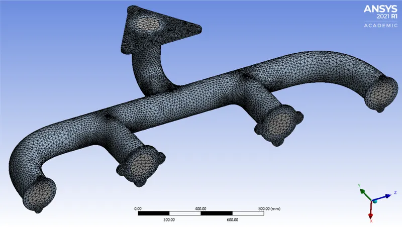
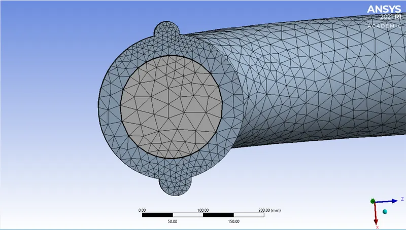
Mesh:

Turbulence Model: K-omega SST

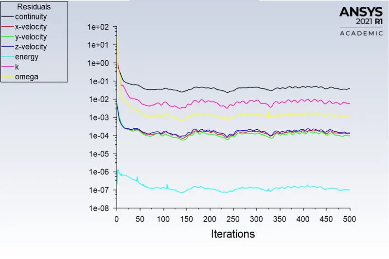
Residual Plot:

Surface Heat transfer Coefficient:

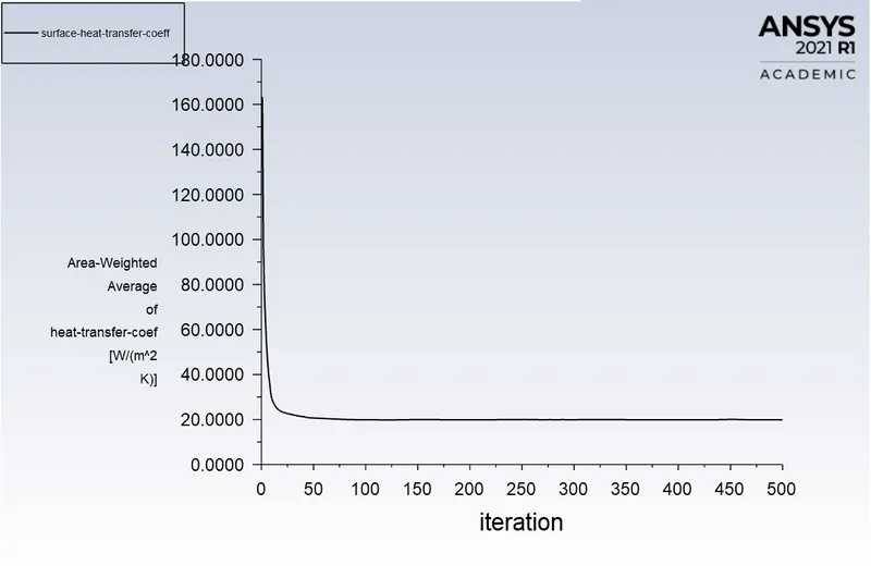
Surface Heat transfer Coefficient = `19.896339 W/m^2 K`

Temperature contour:

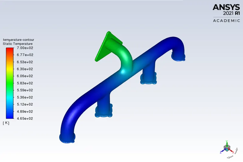
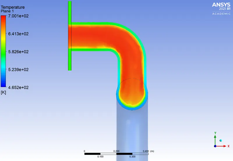
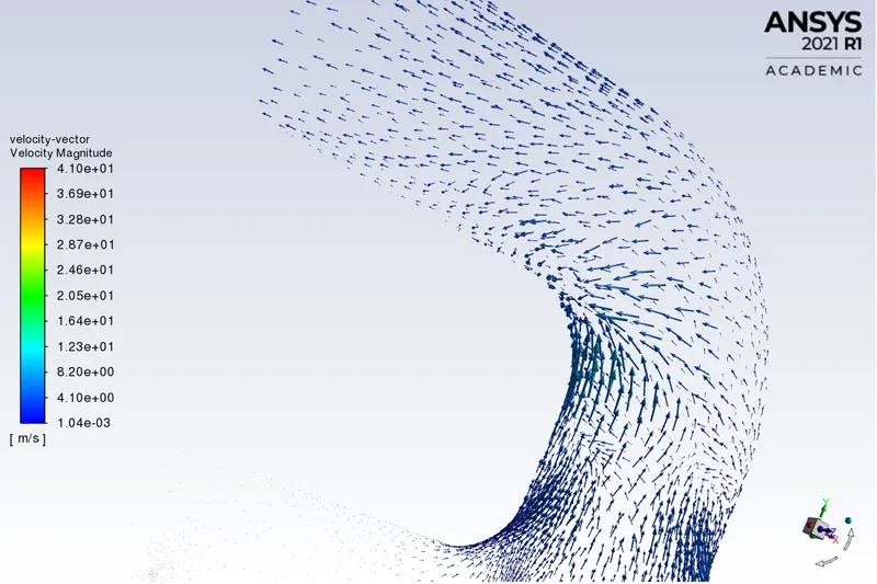
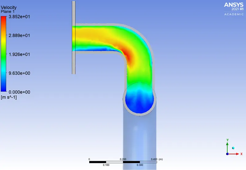
Velocity contour:

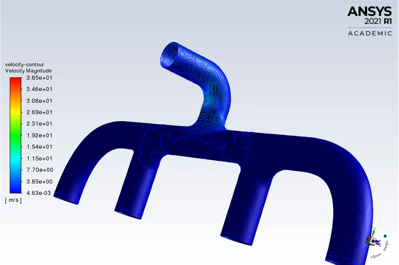
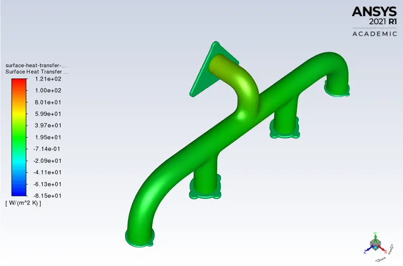
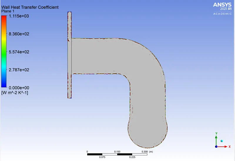
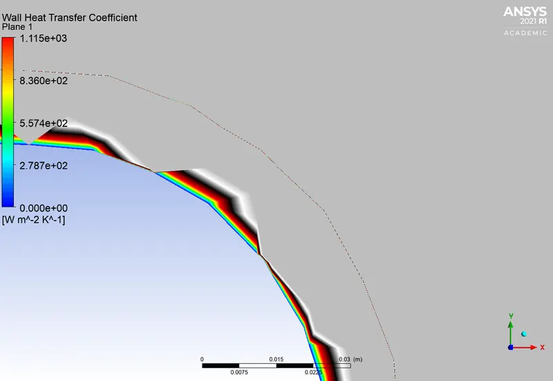
Heat transfer coefficient:

2. When y+ = 30

First layer thickness = 1.7348

Number of inflation layers = 7

Growth rate = 1.2

Total layer thickness = 22.4065

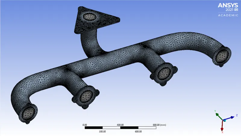
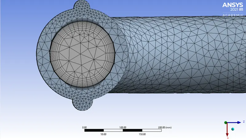
Number of elements = 471639

Mesh:

Turbulence Model: K-epsilon Standard

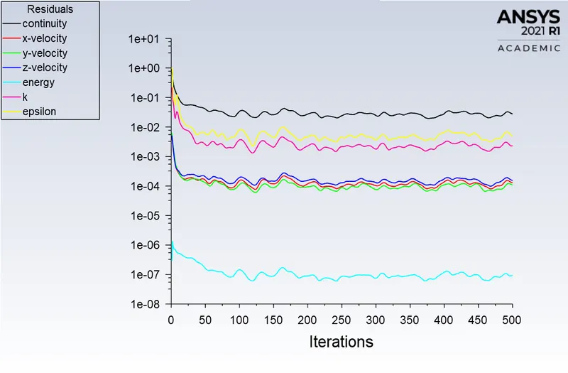
Residual Plot:

Surface Heat transfer Coefficient:

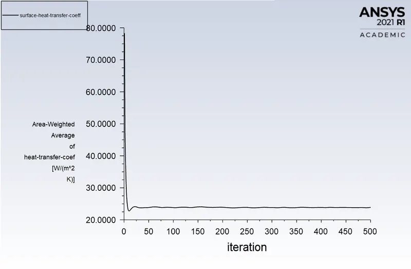
Surface Heat transfer Coefficient = `23.8900 W/m^2 K`

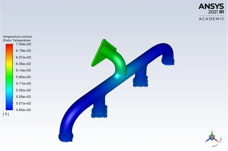
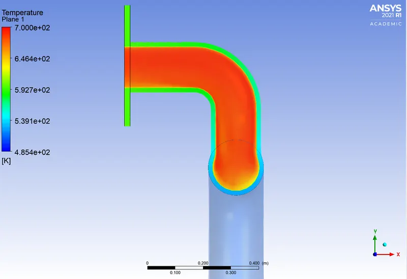
Temperature contour:

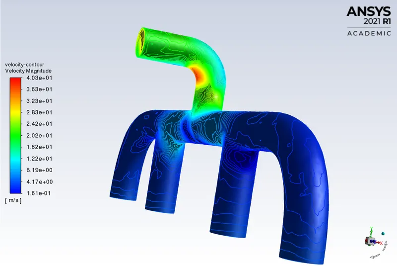
Velocity contour:

Heat transfer coefficient:

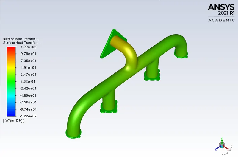
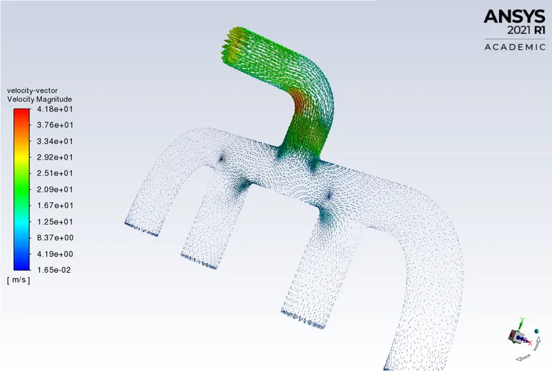
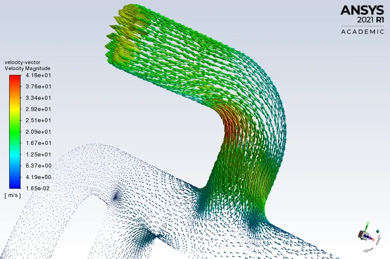
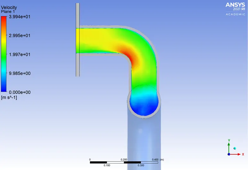
Let's discuss all the contours or results that we are getting here. As we have a hot exhaust port coming in, they are at a high temperature of 700 k. But if we look at the solid metal temperature close to the inlets is around 470-480 k whereas in the place where all the pipes meet the temperature is around 550-560 k this is occurring because of Convection.

The velocity is really low in the inlet sections but the velocity is really high in the outlet section this is because of Mass conservation. As all of these diameters are similar so we can say that the velocity on all these inlet faces is pretty much the same and Area x Velocity is the flow rate, and there are four inlets and only one outlet, all the air needs to flow out which means velocity is going to be high there. Because of this higher velocity, there will have a higher Reynolds number which means we should have a higher heat transfer coefficient which means there is going to be more heat transfer from the fluid to the solid. That is why the solid temperature in that location is higher.

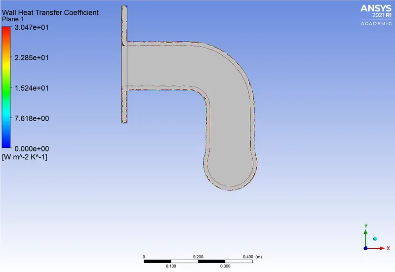
Wall heat transfer coefficient is a quantity that is calculated only at the walls that is why we can see that it is calculated only in the walls that are adjacent to the fluid. We can observe the wall heat transfer coefficient is highest where the velocity is also highest. since the fluid is hot we will have the maximum amount of heat transfer from the fluid to the solid which results in a higher temperature of the solid in that particular location.

It can be seen from the images that by refining the mesh and adding the inflation layers we got a smooth plot at the inner boundary. As we know that the heat transfer coefficient is only available in the first cell that is attached to the wall which can be seen properly in the refined mesh images.

Result Comparision:

						Surface Heat Transfer Coefficient Using Viscous Model
y+ Value	First Layer Thickness (y)	Number of Inflation Layers (N)	Growth Rate (G)	Total Layer Thickness (`y_t`)	Number of Elements	k-omega SST	K-epsilon Standard	k-epsilon Realizable
y+ = 1	0.05782	7	1.2	0.746797	485951	19.8963	-	22.7880
y+ = 2	0.11565	7	1.2	1.4937	498334	22.2789	-	29.3471
y+ = 4	0.2313	7	1.2	2.9874	464388	23.9130	-	31.4518
y+ = 5	0.2891	7	1.2	3.7343	461981	24.2058	-	31.3461
y+ = 30	1.7348	7	1.2	22.4065	471639	25.7155	23.8900	24.4207
y+ = 40	2.3131	7	1.2	29.8757	467010	26.4069	24.3095	24.9888
y+ = 50	2.8913	7	1.2	37.3437	461842	26.6890	24.7087	25.5951
y+ = 60	3.4696	7	1.2	44.8130	459311	26.7866	25.0076	25.74065
y+ = 70	4.0479	7	1.2	52.2822	456244	26.7088	24.9407	26.0640
y+ = 80	4.6262	7	1.2	59.7515	454796	26.8257	24.9796	26.3641
y+ = 90	5.2045	7	1.2	67.2208	455873	26.9677	25.1443	26.4171

K-epsilon model is used where flow does not demand to integrate the solution through the viscous sublayer and wall-bounded effects are secondary. For such cases the first cell away from the wall shall be placed at a y+ of 30-300. In such a scenario, the viscous sublayer and buffer layer are not resolved.

K-epsilon Standard wall function: The lower limit of y+ is 11.225 hence standard wall function should not be used below that limit as the solution accuracy might deteriorate in an uncontrolled manner. we can observe from the above comparison table the solution deteriorated in an uncontrolled manner when the y+ value was given below that limit.

K-omega model can be used where the flow demands integrating through the viscous sublayer include calculation of heat transfer. Integrating through the viscous sublayer would generally impose resolving the mesh to `y+<=1`. The omega equation can be integrated through the viscous sublayer.

The heat transfer coefficient is seen at the very first cell of the wall. The value of the heat transfer coefficient is calculated in the cell adjacent to the wall which allows us to choose the value of y+ = 1 which is in the viscous sublayer and the turbulent model k-omega SST. We can observe from the table when we used the y+ of 1 for the k-omega SST model we got a heat transfer coefficient of `19.8963 W/m^2 K` which is very close to the analytical value which `19.48 W/m^2 K`.

We can also observe that as we increase the y+ value the heat transfer coefficient value is going far from the analytical value of the heat transfer coefficient. So we can conclude that for this particular problem the y+ = 1 with K-omega SST model should be used.

Accuracy of the prediction depends on factors:

• Y+ value: Correct choosing the value of y+ will give a more accurate solution.
• Mesh: Finer mesh gives better results as compared to coarser. The mesh should be conformal.
• Inflation layer: It increases the quality of mesh near the boundary interface and helps to capture smooth plots of different quantities.
• Model: Selecting the right turbulence model according to the y+ value greatly impacts the accuracy of results.