Week-4 Challenge WOT Condition Part-2

___Q1___

What is the difference between mapped and dynamic model of engine, motor and generator? How can you change model type?

	MAPPED MODEL	DYNAMIC MODEL
SETTINGS	It is default system setting.	It needs to be chosen by the user.
DATA	It runs based on data given in standard look up tables.	Data here is specified by ther user. It represents actual components of the system.
RUN TIME	It runs faster and take less simulation time as the system is static.	It is relatively slow and takes more simulation time as it tracks actual components of the system.
ACCURACY	It is less accurate, as it works on experimental data.	It is more accurate, as it works on user defined data.
EXAMPLE	Mapped generator works with maximum torque and speed data.	Dynamic generator works with speed control, torque control, dynamics of 3 phase PMSM, 3 phase inverter etc.

Changing the model type :

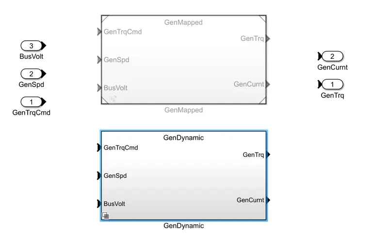
1- Image below shows HEV model.

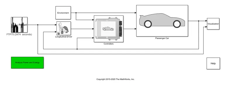
2- Double clicking Passenger Car block --> various blocks (Engine, electric Plant, Drivetrain) --> selecting Electric Plant

--> we see Generator block and Motor Block --> selecting Generator block.

3- By defalut Mapped Generator block is selected.

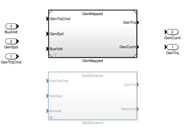
4- To select Dynamic model,

Modelling Tab (matlab window) ---> Design Section (drop down menu) ---> Selecting Variant manager.

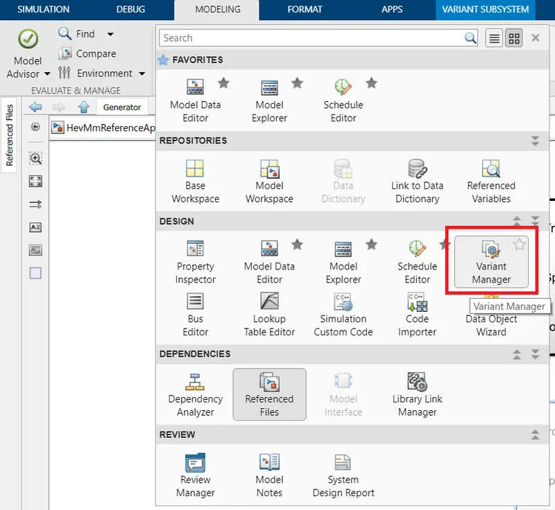
5- In variant manager, various model blocks are listed.

Passenger Car ---> Electric Plant ---> Generator ---> GenDynamic right click ---> setting label to Active mode.

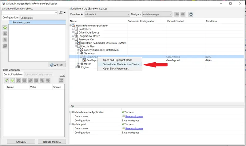
6- Generator changed to Dynamic block. The same process can be repeated for all other blocks.

___Q2___

How does the model calculate miles per gallon? Which factors are considered to model fuel flow?

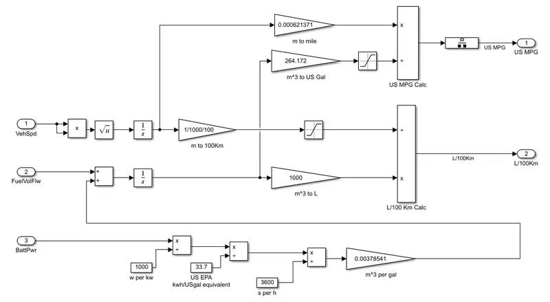
Answer : The model calculate miles per gallon by the following block -

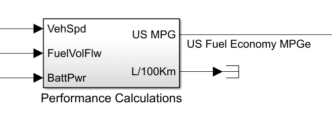
• MPGe stands for Miles per gallon of gasoline-equivalent.
• It was introduced by Environmental Protection Agency (EPA).
• 1 gallon of gasoline = 33.7 kWh of electricity.

• Distance travelled is calculated using vechicle speed in meter then converting to miles.
• Battery power is then converted to W then divided by US EPA i.e. 33.7 to get gasoline equivalent.
• Now dividing Distance travelled in miles by number of gallons (gasoline equivalent) gives miles per gallon.

___Q3___

AIM : To run HEV Reference Application with WOT drive cycle.

GIVEN : Change Grade & Wind Velocity in environment block.

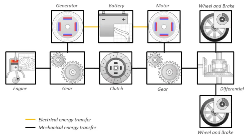
THEORY : HEV model is as follows -

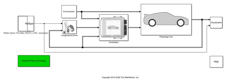
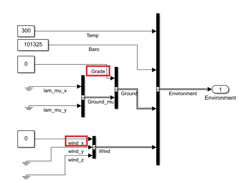
The environment block is modelled as follows -

HEV block Diagram -

For WOT, Step input is applied with

Reference Speed = 50m/s (111 mph).

Deceleration Time = 80 s.

Run Time = 100 s.

OBSERVATION :

1- Grade = 0 & Wind Velocity = 0 m/s.

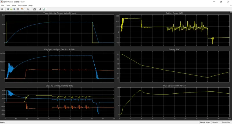
From above plot we can observe that the acceleration time is quite large (40 s) because the power paramaters of the motor are capped in the model. The actual speed eventually follows the reference speed & starts decelerating from 80th second. Similarly we can see the SOC also increasing due to regeneration during deceleration period.

2- Grade = 5, Wind Velocity = 0 m/s.

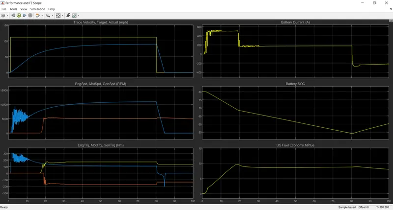
With grade increased, the hill climbing force also increases.

we can see that vehicle is not able to keep up with the reference speed due to less velocity.

3- Grade = 5, Wind Velocity = 10 m/s.

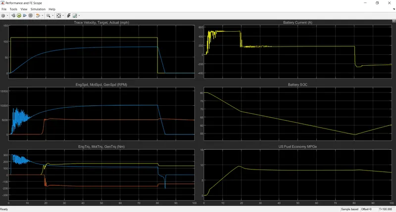
With increased wind velocity, the aerodynamic force also increases.

the peak velocity of the vehicle dips even more and not able to keep up with the reference speed.

CONCLUSION :

In normal conditions the vehicle is eventually following the reference speed, but with increased effect of gradeability and wind velocity the peak velocity of vehicle goes on decreasing due to increased effect of hill climbing force as well as aerodynamic force.

___Q4___

AIM : To compare simulated results of HEV with Pure EV powertrain.

GIVEN : All parameters same for EV powertrain.

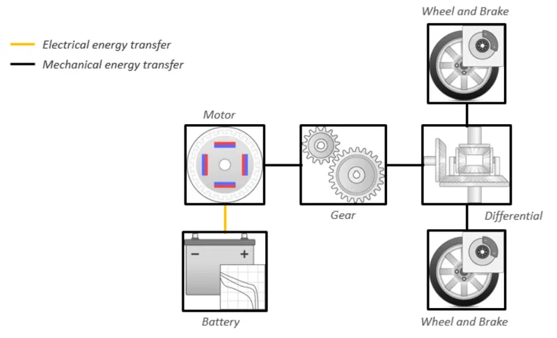
THEORY : EV model is as follows -

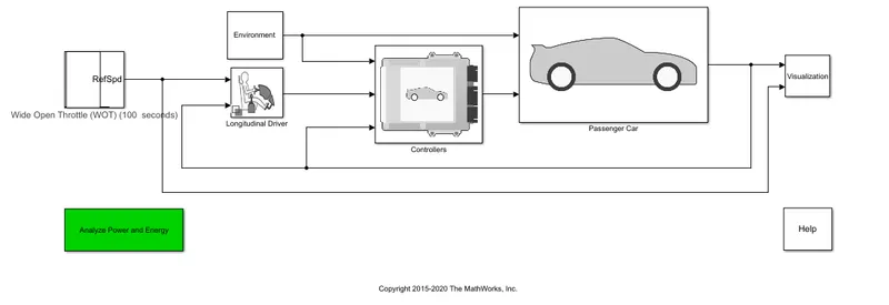
Pure EV Block Diagram -

For WOT, Step input is applied with

Reference Speed = 50m/s (111 mph).

Deceleration Time = 80 s.

Run Time = 100 s.

OBSERVATION :

1- Grade = 0 & Wind Velocity = 0 m/s.

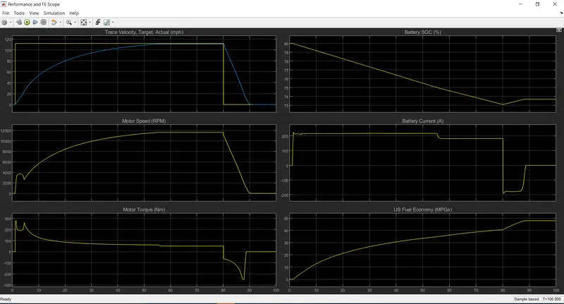
From the above plot we can observe that the acceleration time is even more large than an HEV i.e. 55 s.

But eventually the vehicle speed follow the reference speed.

The increase in SOC during the deceration is also not quite considerable when compared with an HEV.

2- Grade = 5, Wind Velocity = 0 m/s.

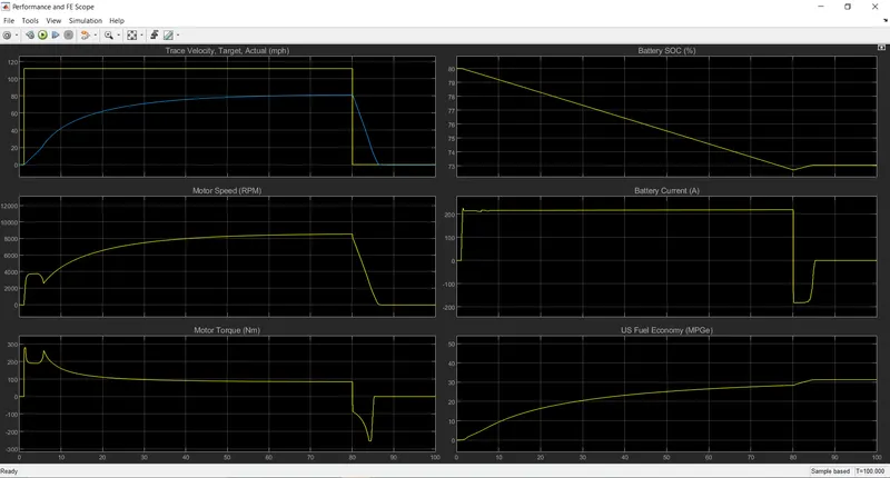
With grade increased, the hill climbing force also increases.

we can see that vehicle is not able to keep up with the reference speed due to less velocity, which is even less when compared with an HEV.

3- Grade = 5, Wind Velocity = 10 m/s.

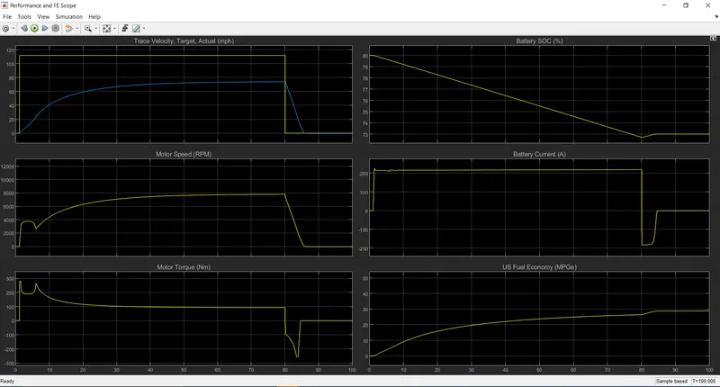
With increased wind velocity, the aerodynamic force also increases.

the peak velocity of the vehicle dips even more as compared with an HEV, and not able to keep up with the reference speed.

CONCLUSION :

	HEV	EV
1- Grade = 0, Wind Velocity = 0 Peak Velocity Decelaration Time SOC change	111 mph 6 sec 5% Increase	111 mph 10.7 sec 0.6% Increase
2- Grade = 5, Wind Velocity = 0 Peak Velocity Decelaration Time SOC change	89 mph 4.4 sec 6% Increase	80 mph 6.8 sec 0.3% increase
3- Grade = 5, Wind Velocity = 10 Peak Velocity Decelaration Time SOC change	82.7 mph 4.14 sec 6% Increase	74 mph 5.9 sec 0.28% Increase
4 - Fuel Economy	Less	More

When Pure EV preformance is compared with an HEV, the peak velocity of EV is lower than an HEV for various conditions.

But the fuel economy for EV is unmatachable with that of HEV.