Week-4 Challenge WOT Condition Part-2

1. The difference between mapped and dynamic model is that:

In a mapped model, pre-entered data (for example, a drive cycle) is used for operation and simulation.

Whereas,

In a dynamic model, analysis and simulation is done according to real time conditions.

As a result,

Time taken for simulation of mapped model is much lesser than that for a dynamic model.

Also, a mapped model would give less accurate results because the operating conditions are already pre-defined in this situation.

But a dynamic model would give very accurate results as it takes into consideration all the real time conditions and parameters.

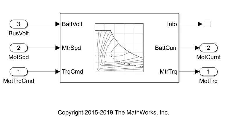
Fig 1: Mapped model block

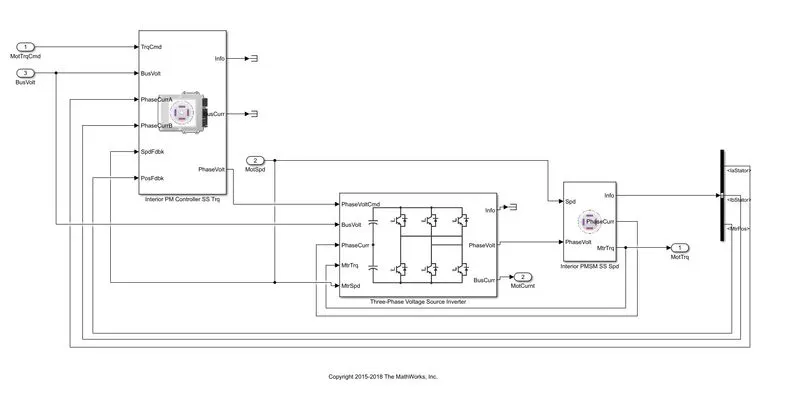
Fig 2: Dynamic model block

In order to change the model type, we have to follow the following steps:

a. Open the model in Simulink.

b. Open the 'Passenger Car' block.

c. Open the 'Electric Plant' block.

d. Right Click on the 'Motor' Block (MotGenEvMapped).

e. Go to 'Variant' -> Label Mode Active Choice -> Select desired model type

2. Miles per gallon is the distance travelled by a vehicle powered by one gallon of gasoline or diesel fuel unit.

According to Environment Protection Agency, the metric to measure the energy consumed by alternative fuel vehicles is MPGe (i.e., Miles per gallon equivalent). This is obtained by calculating the amount of electricity required to produce the same amount of heat (=115000 BTUs) that is produced by burning a gallon of gasoline. The electricity equivalent thus achieved is 33.7 kilowatt hour.

i.e, a electric vehicle that can travel 100 miles on 33.7 kWh of electricity has an energy consumption of 100 MPGe.

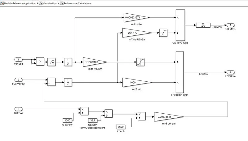
Fig 3:MPG block

Here, from the Performance Calculations block, we can see that there are three inputs considered for the calculation of US MPG:

a. Vehicle speed

Vehicle speed input is takenand multiplied with itself and then its square root is taken. This value is integrated over time to obtain the distance in meters (m). The distance obtained is then converted to miles by multiplying with a factor of 0.000621371.

b. Battery power

We have the following equations:

264.172 US Gallon = 1000L and
1 Gallon = 33.7 kWh

The battery power input is taken and divided by 1000 and then by 33.7 to obtain the US EPA/US Gallon equivalent. It is then divided by 3600 and converted to m^3 per gallon by multiplying with a factor of 0.00378541 (Since, 1 US Gallon = 0.00378541 m^3)

In case of Hybrid electric vehicles, there is another factor considered:

c. Battery power

This input is added along with battery power input and then integrated. This value is then multiplied by 1000 to obtain the value in liters (L) or by 264.172 to obtain the value in US Gallon.

The factors that we need to consider while modelling fuel flow are that:

a. It is difficult to estimate HEV fuel consumption because of the complexity of both ICE and EV components.

b. Fuel consumption rates are significantly affected by vehicle speed and acceleration rates.

c. So, when an HEV should be able to run only on the electric motor when the power required is less, in order to obtain better fuel consumption figures.

3. To obtain the performance plots after the simulation, we can open the Performance and FE Scope in the 'Visualization' block as shown below:

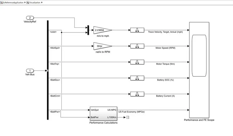
Fig 4: Visualization Block

First we simulate the WOT cycle with the default settings. In the Drive Cycle Setup, we set up the cycle for 100 seconds where full throttle is given at 5 seconds and removed at 50 seconds. The plot obtained is portrayed below:

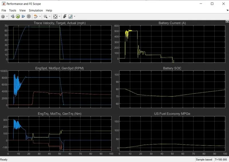
Fig 5: Default WOT plot

In this plot we can see that the vehicle needs 12.273 seconds to accelerate from 0 to 67.4 mph
During this period the Battery SOC drops from 80% to 72.37%.

Next, we change the wind velocity value to 10 and run the simulation again. The plot obtained is given below:

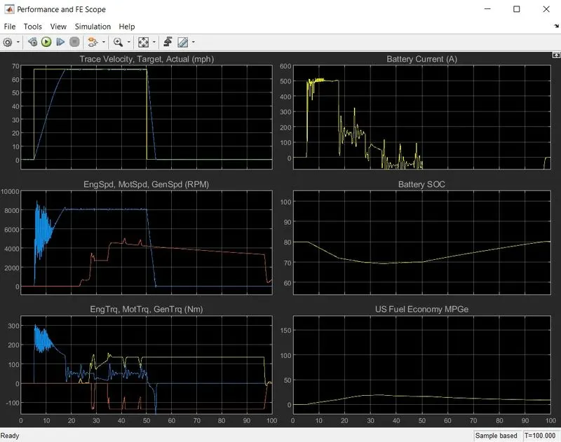
Fig 6: WOT plot with wind velocity 10

In this plot we can see that the vehicle needs 12.786 seconds to reach the maximum velocity of 67.4 mph.
The battery SOC drops from 80% to 71.94%.

Now, we change the wind velocity value back to 0 and change the grade to 10 and re-run the simulation. The plot obtained is given below:

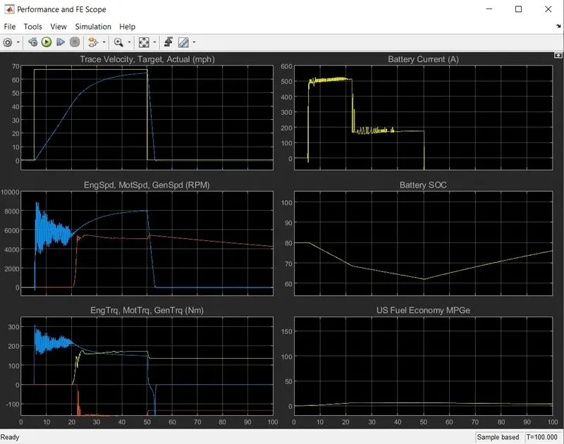
Fig 7: WOT plot for grade 10

In this plot we can see that for the 45 seconds that the vehicle is accelerated, it does not reach the maximum velocity. It manages to reach a maximum velocity of 64.5 mph.
Battery SOC drops from 80% to 62.09% during this entire time.

For the last simulation, we keep both the grade value and the wind velocity value to 10 and run the simulation and obtain the plot:

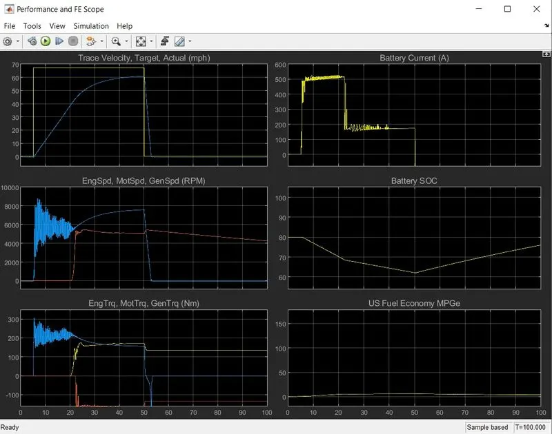
Fig 8: WOT plot for wind velocity 10 and grade 10

In this plot we can see that the vehicle accelerates from 0 to 60.9mph in 45 seconds. And the battery SOC drops from 80% to 62.11% during the process.

CONCLUSION:

We can see that the wind velocity that we have considered does not affect the vehicle to a huge extent, but the grade has a fairly large impact on the performance of the vehicle.

4. Below are the plots of WOT drive cycle of EV and HEV drivetrains under default conditions. Cycle is simulated for 100 seconds wherein throttle is removed after 50 seconds.

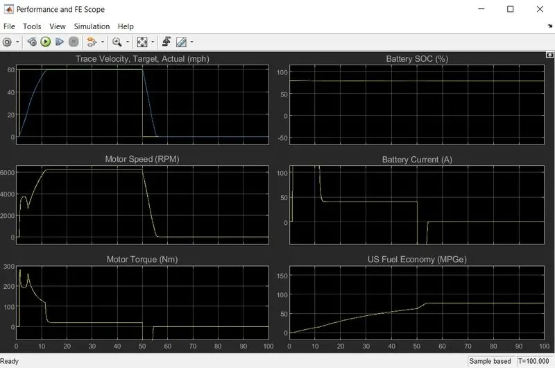
Fig 9: Performance plot for EV

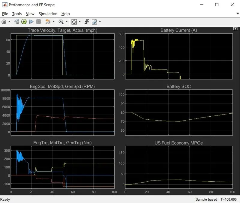
Fig 10: Performance plot for HEV

From the plots we arrive at the following conclusions:

a. EV drivetrain achieves a top speed of 60mph whereas HEV drivetrain achieves a top speed of 67.4 mph.

b. Fuel Economy is higher for the EV because of a completely electric drivetrain.

c. Motor speed (RPM) graph is much smoother in case of EV because of the much simpler working of the drivetrain. The HEV, on the other hand, is very jagged due the complexities of having both an electric motor and a combustion engine.