Week 4.1 - Genetic Algorithm

What is Genetic Algorithm?

Genetic algorithm is an optimisation method based on random sampling following the concepts of genetics and natural selection. It is inspired by Darwin's theory of natural evolution where in the fittest individuals are selected to reproduce and form offsprings for the next generation. These offsprings will be fitter and more likely to survive among the others whose parents were not among the fittest in the previous generation.

In MATLAB, genetic algorithm consists of 5 phases:
1. Initial population

2. Fitness function

3. Selection

4. Crossover

5. Mutation

First, the algorithm selects a random collection of solutions. These solutions are then evaluated by a fitness function, where the ones with better fitness will be able to breed and produce the next generation. Randomly, mutation may occur that may alter the genetic structure of the parents, thus adding to the variability. What was first started as a random population would then turn into a population selected by better fitness characteristics. After several iterations, we would arrive at an optimum value.

Syntax of ga:

[x, fval] = ga(func, nvars, A, b, Aeq, beq, lb, ub, nonlcon, options)

where,

ga=genetic algorithm

func = function call

nvars = number of variables

A = Linear inequality constraints, specified as a real matrix

b = Linear inequality constraints, specified as a real vector

Aeq = Linear equality constraints specified as a real matrix

beq = Linear equality constraints specified as a real vector

lb = lower bound

ub = upper bound

nonlcon = non linear constraints, specified as function handle

options = optimisation options, specified as the output

Main Code:

clear all
close all
clc

%defining out search space
x=linspace(0,0.6,150);
y=linspace(0,0.6,150);
num_cases = 50

%Creating a 2Dimensional mesh
[xx yy] = meshgrid(x,y);

%Evaluating the stalagmite function
for i=1:length(xx)
    for j=1:length(yy)
          input_vector(1)=xx(i,j);
          input_vector(2)=yy(i,j);
          f(i,j)=stalagmite(input_vector);
    end
end


%Study 1 - Statistical behaviour
%initiating tic-toc counter to mesasure the time taken to run the genetic algorithm
tic
for i = 1:num_cases
    [inputs, fopt(i)] = ga(@stalagmite,2);
    xopt(i) = inputs(1);
    yopt(i) = inputs(2);    
end

time1=toc

figure(1)
%subplot(m,n,p) divides the figure window into m x n grid
%and p is our desired position of the plot
subplot(2,1,1)
hold on
%visualising the function
surfc(x,y,-f)
%removing gridlines from the plot
shading interp
%using plot3 command for 3D plotting the optimum values
plot3(xopt,yopt,-fopt,'marker','o','markersize',5,'markerfacecolor','r')
title('Unbounded inputs')
xlabel('x values')
ylabel('y values')
%plotting optimum values predicted by the function against the iterations
subplot(2,1,2)
plot(-fopt)
xlabel('Iterations')
ylabel('Function maximum')



%Study 2 - Statistical behaviour - with upper and lower bounds
tic
for i=1:num_cases
    [inputs, fopt(i)] = ga(@stalagmite,2,[],[],[],[],[0;0],[1;1]);
        xopt(i)=inputs(1);
        yopt(i)=inputs(2);
end

time2=toc

figure(2)
%subplot(m,n,p) divides the figure window into m x n grid
%and p is our desired position of the plot
subplot(2,1,1)
hold on
%visualising the function
surfc(x,y,-f)
%removing gridlines from the plot
shading interp
%using plot3 command for 3D plotting the optimum values
plot3(xopt,yopt,-fopt,'marker','o','markersize',5,'markerfacecolor','r')
title('Bounded inputs')
xlabel('x values')
ylabel('y values')
%plotting optimum values predicted by the function against the iterations
subplot(2,1,2)
plot(-fopt)
xlabel('Iteration')
ylabel('Function maximum')

%Study 3 - Increasing GA iterations
options = optimoptions('ga');
%in this we shall increase our population size in order to achieve better
%results from the genetic algorithm
options = optimoptions(options,'PopulationSize',300);

tic
for i = 1:num_cases
    [inputs,fopt(i)]=ga(@stalagmite,2,[],[],[],[],[0;0],[1;1],[],[],options);
    xopt(i) = inputs(1);
    yopt(i) = inputs(2);
end
time3=toc

figure(3)
%subplot(m,n,p) divides the figure window into m x n grid
%and p is our desired position of the plot
subplot(2,1,1)
hold on
%visualising the function
surfc(x,y,-f)
%removing gridlines from the plot
shading interp
%using plot3 command for 3D plotting the optimum values
plot3(xopt,yopt,-fopt,'marker','o','markersize',5,'markerfacecolor','r')
title('Bounded inputs with increased population size')
xlabel('x values')
ylabel('y values')
%plotting optimum values predicted by the function against the iterations
subplot(2,1,2)
plot(-fopt)
xlabel('Iteration')
ylabel('Function maximum')

where our stalagmite function is defined as:

function [f]= stalagmite(input_vector)

x= input_vector(1);
y= input_vector(2);

f1_x = (sin(5.1*pi*x + 0.5))^6;
f1_y = (sin(5.1*pi*y + 0.5))^6;
f2_x = exp((-4*log(2)*(x - 0.0667)^2)/0.64);
f2_y = exp((-4*log(2)*(y - 0.0667)^2)/0.64);

[f]=-(f1_x*f1_y*f2_x*f2_y);

Results obtained:

Study 1:

Study 2:

Study 3:

Explanation:

1. We clear all graphs or plots and initially define our search space (x and y) using linspace. Then we use the meshgrid command to create a 2D mesh from x and y.

2. This 2D mesh will provide us the input for our stalagmite function, which will evaluate the fitness values for the given inputs.

3. We will then use the 'ga' function to optimise the stalagmite function and try to obtain our maxima.

The optimised output will be stored as 'fopt' and the corresponding values of x and y wil be stored as 'xopt' and 'yopt'.

A. Study 1:

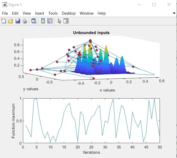
Here, the 'ga' function runs for 50 iterations. This study is unbounded, i.e, the 'ga' function does not have any limitation to its search space. This gives a wide range of solutions which may need to be optimised again.

B. Study 2:

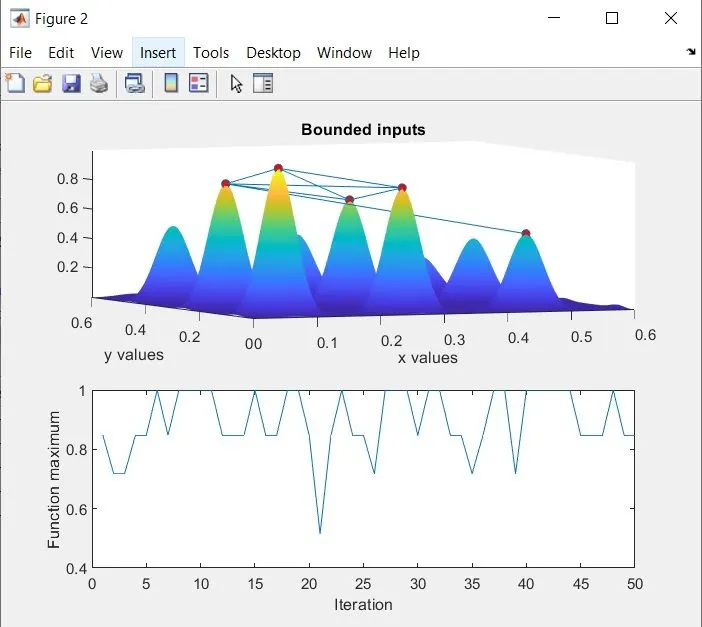
Here, the 'ga' function runs for 50 iterations. This study has limited the search space for the 'ga' function to in between 0 and 1 for both x and y. Here, the solutions are narrowed down to a small number and hence gives better results than the previous study.

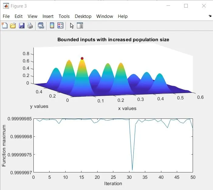
C. Here too the 'ga' function runs for 50 iterations but in this case, the population size has been increased to 300. This study finally gives us a single solution to our global maxima, or in certain cases 2 and thus we can get the optimised result from this study.

In these studies, we have also used the tic-toc command to calculate the time taken for the ga to process the data. tic starts the timer and toc stops it. The time taken for each study has also been recorded.

Finally after each study a surface plot using the 'surfc' command is drawn where we can visually represent the solutions obtained. Also a subplot showing the values obtained for each iteration is also plotted alongside.

Changes made to the stalagmite function:

The ga function is coded to provide us with minima. So, in order to obtain the maxima in our studies we add a negative sign to the outputs provided by it. Hence while plotting we plot '-fopt' instead of 'fopt'.

Similarly in the stalagmite function too, we add a negative sign to the value returned by the function.

References:

https://in.mathworks.com/discovery/genetic-algorithm.html