Week 3 - Solving second order ODEs

Introduction:

The equation representing the motion of simple pendulum with damping is defined as:

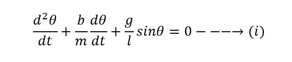
For solving a second order differential equation in MATLAB, we first break it down into a first order differential equation.

Lets consider,

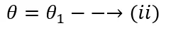
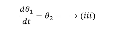
This gives us equation (i) as:

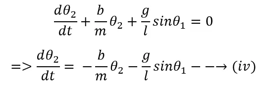
We are given the following parameters:

length of pendulum wire, l=1m

mass of pendulum, m=1kg

damping coefficient, b= 0.05

gravity, g=9.81 m/s^2

At time t=0, angular displacement = 0 and angular velocity = 3 rad/s

Code:

clear all
close all
clc

%using ode (d/dt)^2*(theta) + (b/m)*(d/dt)*(theta) + (g/l)*sin(theta) = 0

b=0.05; 
m=1; %kg
g=9.81; %m/s^2
l=1; %m

%initial condition
%i.e. at (theta=0) the displacement of the pendulum was 0 and the velocity
%was 3 rad/s
theta_0=[0,3];

%time array
t_span=linspace(0,20,500);

%ode45 is an enabled solver in matlab for ordinary differential equations
%SOLVE ODE
[t,results]=ode45(@(t,theta) ode_func(t,theta, b, m, g, l), t_span, theta_0);

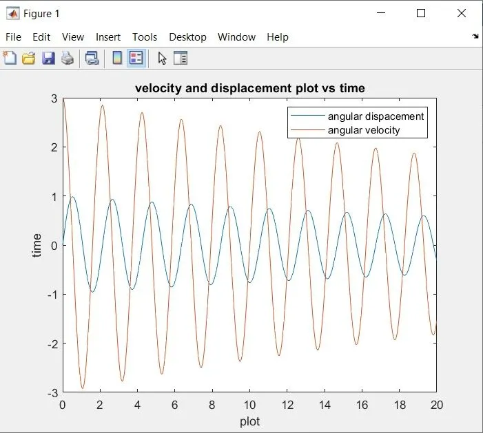
plot(t, results(:,1))
hold on
plot(t, results(:,2))
title('velocity and displacement plot vs time')
xlabel('plot')
ylabel('time')
legend('angular dispacement','angular velocity')

theta_1=results(:,1);
ct=1; %initiating counter

%pendulum hinge coordinates
x0=0; 
y0=0;

%for-loop for the animation
for i=1:length(theta_1)
    theta_2=theta_1(i);
   
    %free end of pendulum for each instance
    x1=l*sin(theta_2);
    y1=-l*cos(theta_2);
    
    %plotting
    figure(2)
    plot([-2 2],[0 0],'linewidth',5) %plotting fixed wall from which pendulum is hanged
    hold on
    plot(x1,y1,'.','markersize',40) %plotting free end/bob of the pendulum
    hold on
    plot([x0 x1],[y0 y1]) %plotting pendulum wire
    hold off
    title('damped pendulum animation')
    axis([-3 3 -3 3]) %defining a fixed axis to view the animation properly
    pause(0.01) %frame interval
    
    M(ct)=getframe(gcf) %capturing frame into array M
    ct=ct+1; %incrementing counter
    
end

%saving the animation
movie(M)
videofile=VideoWriter('damped_pendulum.avi','Uncompressed AVI')
open(videofile)
writeVideo(videofile,M)
close(videofile)

where, ode_func is a function defined as

function [dtheta_dt]= ode_func(t,theta,b,m,g,l)

%defining theta1 and theta2 as explained in the derivation
theta1= theta(1)
theta2= theta(2)
dtheta1_dt=theta2;
dtheta2_dt=-(b/m)*theta2  - (g/l)*sin(theta1);
dtheta_dt=[dtheta1_dt;dtheta2_dt];
end

Explanation:

The ode45 is an inbuilt solver to solve the differential equation. Here, ode45 is function of time (t) and angle (theta) which are our primary variables. We have divided the time interval of 20 seconds into 500 equal intervals in the form of a row array and the function call of ode_func provides us with the angular velocity and angular displacement for each interval. This is provided in the form a column array, where the first column provides the angular displacement and the second column gives us the angular velocity.

In order to create the animation, we need to use the for-loop command. We set the loop to start at 1 and go on till the entire length of the 'results' array. The hinge point of the pendulum has been fixed at (0,0) and for each instance in the loop we need to define the coordinates of the free end of the pendulum. This is done by using the command line x1=l*sin(theta_2) and y1=-l*cos(theta_2), where theta_2 is the angle made by the pendulum with the vertical at that instance.

Each of these frames are then captured into an array M using the getframe command. The counter variable is incremented by 1 per loop.

These frames are then put together using the movie command to get the required animation.

Results:

The obtained animation can be checked in the following link:

https://drive.google.com/file/d/1zCB5H8HP_zaN0XB8TvtQyNOG76Z30Tid/view?usp=sharing