Project 2 - Rankine cycle Simulator
What is a Rankine Cycle?
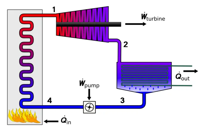
- A rankine cycle closely describes the process by which steam-operated heat engines commonly found in thermal power generation plants generate power. It involves four processes:
1. Process 1-2 (Isentropic compression in pump):
The working fluid is pumped from low to high pressure. As the fluid is liquid at this stage, the pump requires little input energy.
2. Process 2-3 (Constant pressure heat addition in boiler):
The high pressure liquid enters a boiler where it is heated at constant pressure by external heat source to become a dry saturated vapour. The input energy required can be easily calculated graphically, using steam tables.
3. Process 3-4 (Isentropic expansion in turbine):
The dry saturated vapour expands through a turbine, generating power. This decreases the temperature and pressure of the vapour and some condensation may occur. The output in this process can be easily calculated using the steam tables.
4. Process 4-1 (Constant pressure heat rejection in condenser):
The wet vapour then enters a condenser where it is condensed at a constant pressure to become a saturated liquid.
This cycle is graphically represented in the following diagram:
Code:
clear all
close all
clc

%user inputs

fprintf("              RANKINE CYCLE SIMULATOR               \n");
fprintf("1-2 is isentropic expansion in the turbine\n");
fprintf("2-3 is constant pressure heat rejection by the condenser\n");
fprintf("3-4 is isentropic compression in the pump\n");
fprintf("4-1 is constant pressure heat addition by the boiler\n");

p1 = input("Enter the pressure at the turbine inlet (in bar): ");
t1 = input("Enter the temperature at the turbine inlet (in degC): ");
p2 = input("Enter the pressure at the condenser (in bar): ");

%calculating the state point variables

%state 1
h1 = XSteam('h_pT',p1,t1);
s1 = XSteam('s_pT',p1,t1);

%state 2
s2 = s1;
sf2 = XSteam('sL_p',p2);
sg2 = XSteam('sV_p',p2);
sfg2 = sg2 - sf2;
hf2 = XSteam('hL_p',p2);
hg2 = XSteam('hV_p',p2);
hfg2 = hg2 - hf2;
x2 = ((s2-sf2)/sfg2);
h2 = hf2+(x2*hfg2);
t2 = XSteam('T_ps',p2,s2);
t2_sat = XSteam('Tsat_p',p2);


%Calculating turbine work
Wt = h1-h2;

%state 3
p3 = p2;
h3 = XSteam('hL_p',p3);
s3 = XSteam('sL_p',p3);
v3 = XSteam('vL_p',p3);
t3 = XSteam('Tsat_p',p3);

%state 4
p4 = p1;
s4 = s3;
cp4 = XSteam('Cp_ps',p4,s4);
cv4 = XSteam('Cv_ps',p4,s4);
gamma = cp4/cv4;
term1 = (gamma-1)/gamma;
t4 = t3*((p4/p3)^term1);

%Calculating pump work
Wp = v3*(p4-p3)*100;
h4 = h3+Wp;

%Calculating net work, heat addition, heat rejection, thermal efficiency,
%backwork ratio and specific steam consumption
Wnet = Wt-Wp;
Qin = h1 - h4;
Qout = h2 - h3;
T_effi = (Wnet / Qin) * 100;
bw_ratio = Wp/Wt;
ssc = 3600/Wt;


%Plotting the graphs
temp = linspace (1,t1,400);

figure(1)

for i = 1:length(temp)
    s_l(i) = XSteam('sL_t',temp(i));
    s_v(i) = XSteam('sV_t',temp(i));
end
hold on
plot(s_l,temp,'color','r');
plot(s_v,temp,'color','b');
plot([s1,s2],[t1,t2],'color','g');

%if steam at turbine exit is superheated
if t2>t2_sat
    plot([s2,sg2],[t2,t2_sat],'color','y');
    plot([sg2,s3],[t2_sat,t3],'color','y');
else
    plot([s2,s3],[t2,t3],'color','y');
end

plot([s3,s4],[t3,t4],'color','m');

%plotting heat addition in boiler by dividing it into sections
t_boiler_1 = XSteam('Tsat_p',p4);
s_boiler_1 = XSteam('sL_T',t_boiler_1);
plot([s4,s_boiler_1],[t4,t_boiler_1],'color','c');

t_boiler_2 = t_boiler_1;
s_boiler_2 = XSteam('sV_T',t_boiler_2);

plot([s_boiler_1,s_boiler_2],[t_boiler_1,t_boiler_2],'color','c');
plot([s_boiler_2,s1],[t_boiler_2,t1],'color','c');
plot(s1,t1,'.','color','k');
plot(s2,t2,'.','color','k');
plot(s3,t3,'.','color','k');
plot(s4,t4,'.','color','k');

%marking the state points in the plot
text(s1,t1,' 1','color','k');
text(s2,t2,' 2','color','k');
text(s3-0.25,t3,' 3','color','k');
text(s4-0.2,t4,' 4','color','k');
xlabel('Entropy (kJ/kgK)');
ylabel('Temperature (degC)');
title('t-s diagram');
legend('saturated liquid line','saturated vapour line','1-2: isentropic expansion in turbine','2-3: constant pressure heat rejection in condenser','3-4: isentropic compression in pump','4-1: constant pressure heat addition in boiler');

figure(2)
hold on
for j = 1:length(temp)
    h_l(j) = XSteam('hL_T',temp(j));
    h_v(j) = XSteam('hV_T',temp(j));
end
plot(s_l,h_l,'color','r');
plot(s_v,h_v,'color','b');


plot([s1,s2],[h1,h2],'color','g');

%if steam at turbine exit is superheated
if t2>t2_sat
    plot([s2,sg2],[h2,hg2],'color','y');
    plot([sg2,s3],[hg2,h3],'color','y');
else
    plot([s2,s3],[h2,h3],'color','y');
end
plot([s3,s4],[h3,h4],'color','m');
plot([s4,s1],[h4,h1],'color','c');

%marking the state points in the plot
text(s1,h1,' 1','color','k');
text(s2,h2,' 2','color','k');
text(s3,h3,' 3','color','k');
text(s4,h4,' 4','color','k');

xlabel('Entropy (kJ/kgK)');
ylabel('Enthalpy (kJ/kg)');
title('h-s diagram');
legend('saturated liquid line','saturated vapour line','1-2: isentropic expansion in turbine','2-3: constant pressure heat rejection','3-4: isentropic compression in pump','4-1: constant pressure heat addition in boiler');

%displaying the results
fprintf('RESULTS\n')
fprintf('At state point 1: \n')
fprintf('P1 is : %f Bar \n',p1)
fprintf('T1 is : %f Deg Celsius \n',t1)
fprintf('H1 is : %f kJ/kg \n',h1)
fprintf('S1 is : %f kJ/kgK \n\n',s1)

fprintf('At state point 2: \n')
fprintf('P1 is : %f Bar \n',p2)
fprintf('T1 is : %f Deg Celsius \n',t2)
fprintf('H1 is : %f kJ/kg \n',h2)
fprintf('S1 is : %f kJ/kgK \n',s2)
fprintf('X2 is : %f \n\n',x2)

fprintf('At state point 3: \n')
fprintf('P1 is : %f Bar \n',p3)
fprintf('T1 is : %f Deg Celsius \n',t3)
fprintf('H1 is : %f kJ/kg \n',h3)
fprintf('S1 is : %f kJ/kgK \n\n',s3)

fprintf('At state point 4: \n')
fprintf('P1 is : %f Bar \n',p4)
fprintf('T1 is : %f Deg Celsius \n',t4)
fprintf('H1 is : %f kJ/kg \n',h4)
fprintf('S1 is : %f kJ/kgK \n\n',s4)

fprintf('Wt is : %f kJ/kg\n',Wt)
fprintf('Wp is : %f kJ/kg\n',Wp)
fprintf('Wnet is : %f kJ/kg\n',Wnet)
fprintf('Ntherm is : %f percent\n',T_effi)
fprintf('S.S.C is : %f kg/kWh\n',ssc)
fprintf('Backwork ratio: %f\n',bw_ratio)
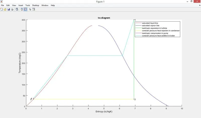
T-S plot:
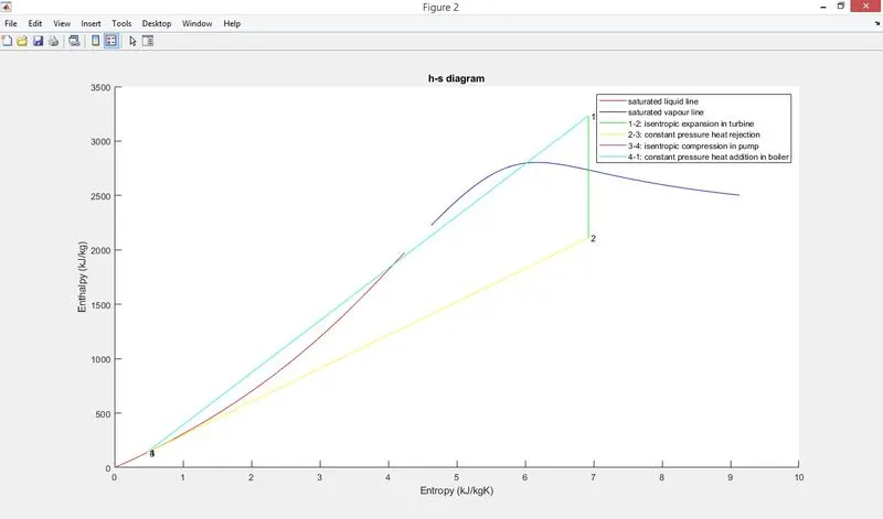
H-S plot:
Explanation:
1. Initially the program asks for input from the user regarding the turbine inlet temperature, turbine inlet pressure and condenser inlet pressure, which in this case were given to be 400 degree celsius, 30 bar and 0.05 bar respectively.
2. We name the states from to 1 to 4 starting from the turbine inlet. We name the variables according to standard nomenclature i.e, h,s,t,p for enthalpy, entropy, temperature and pressure respectively.
3. The user provided inputs are p1, t1 and p2. Using the three given inputs, we calculate the values of the state variables for all the points using the XSteam library.
4. The variable 'sg' and 'sf' refer to saturated vapour and saturated liquid entropies and 'hg' and 'hf' refer to saturated vapour and saturated liquid enthalpies.
5. Once we have calculated the state variables of all the states. We can now calculate the turbine work, pump work, heat addition, heat rejection, net work, thermal efficiency, backwork ratio and specific steam consumption from the mathematical relations known to us.
6. After obtaining the above results, we now plot the t-s diagram of the cycle. For this, we first plot the saturated vapour and saturated liquid lines by dividing the temperature range into an appropriate number and calculating the corresponding entropy values from the XSteam library.
7. Then we plot the state points and join them to obtain our desired plot. We use the 'text' command to number the state points.
8. Similarly, for the h-s plot we divide the temperature range into an appropriate number and obtain corresponding entropy and enthalpy values to plot the saturated liquid and saturated vapour lines. We plot the state points and join them to obtain our desired plot.
9. In addition we make a code that takes into consideration situations where the steam may be superheated at the turbine outlet. This code would then join the point 2 to the saturated vapour line before joining it to the point 3.
10. Finally using 'fprintf' we display the results of each individual state.